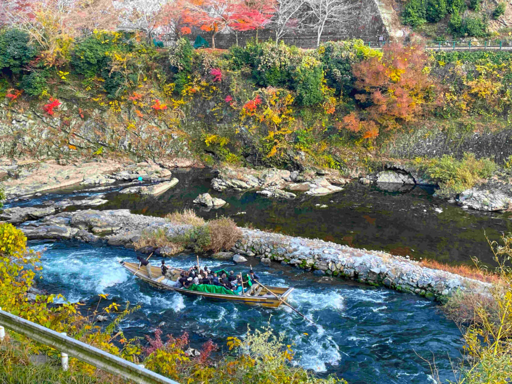
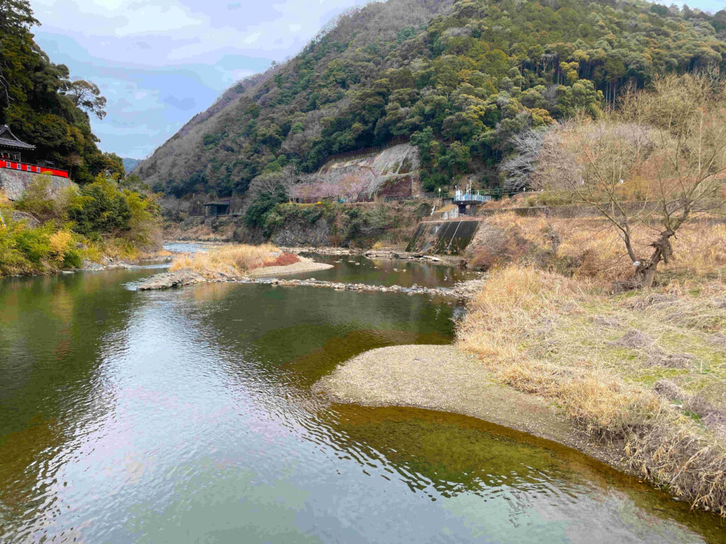
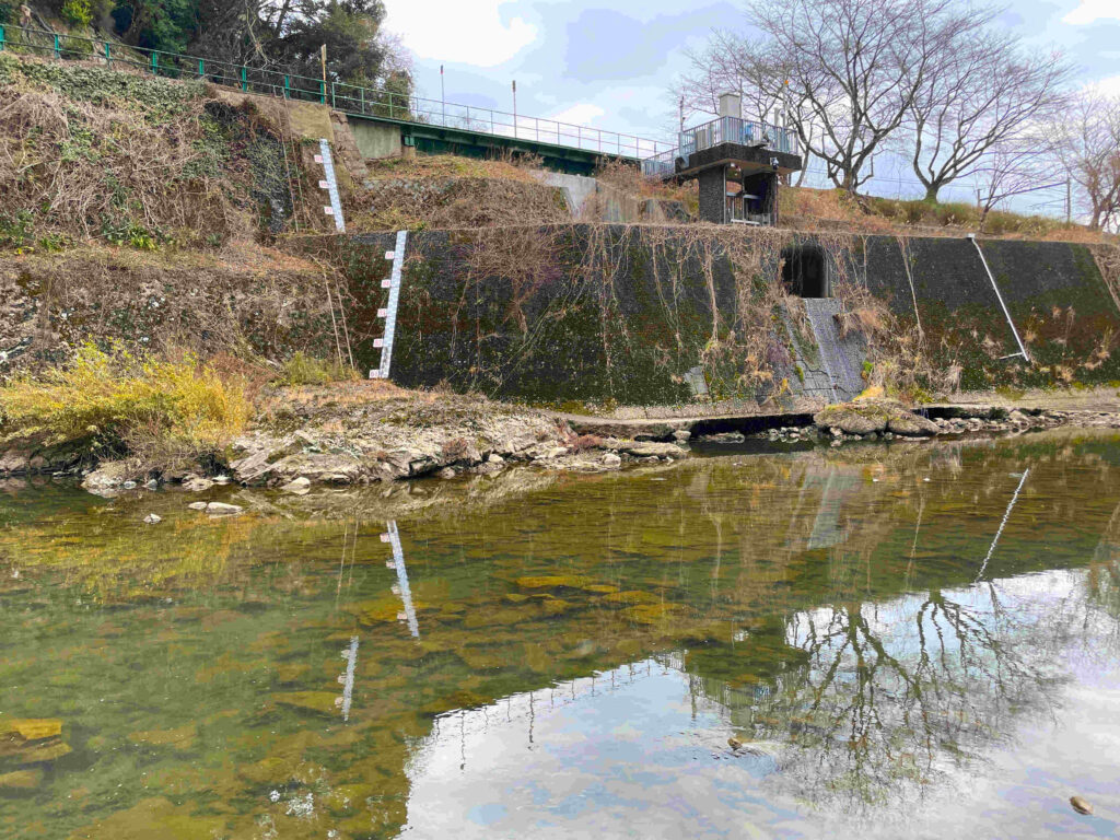
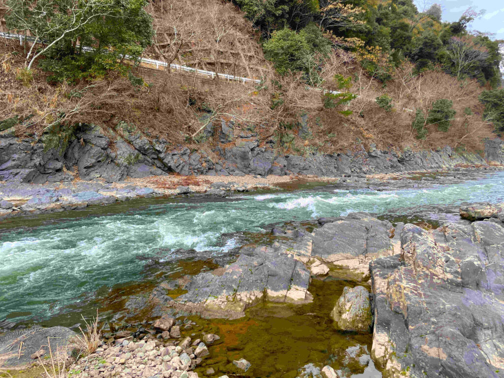
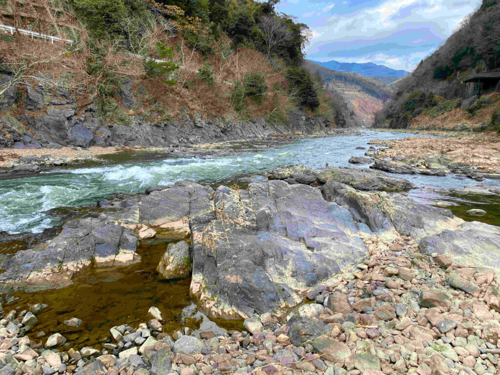
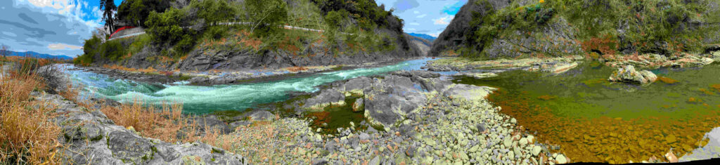
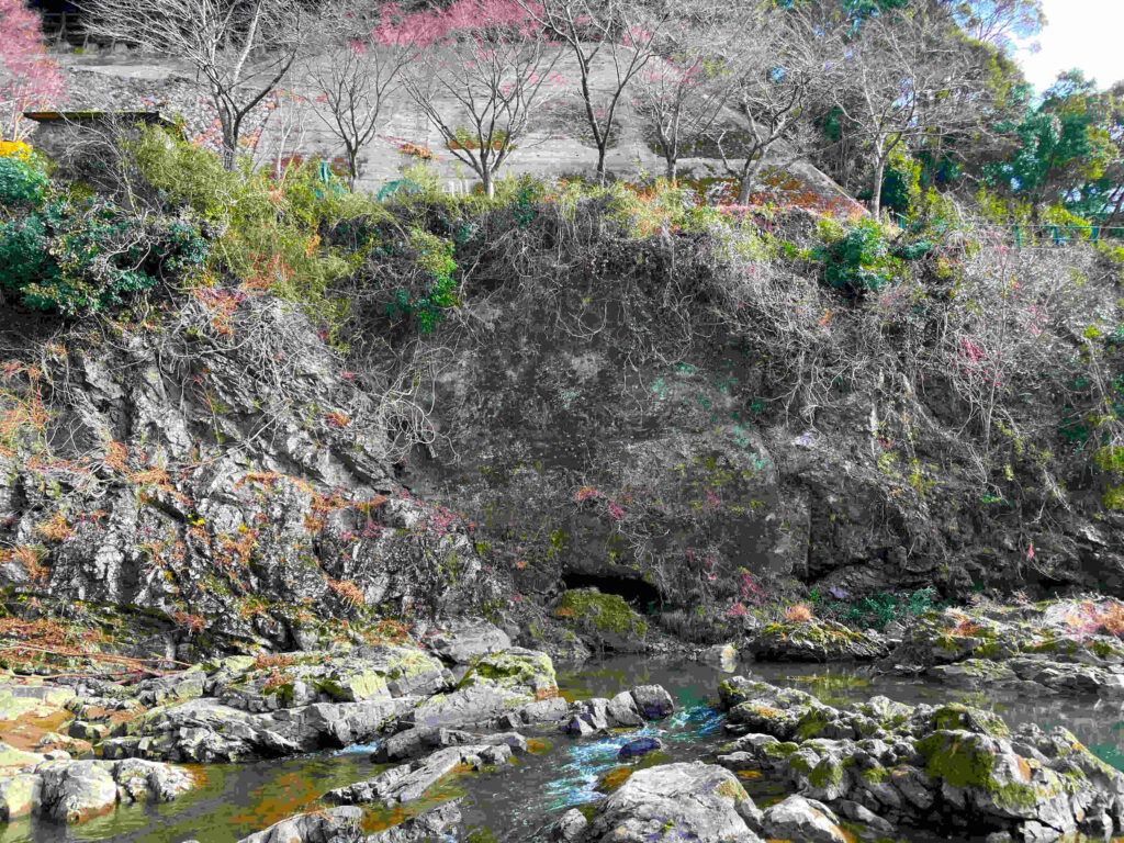
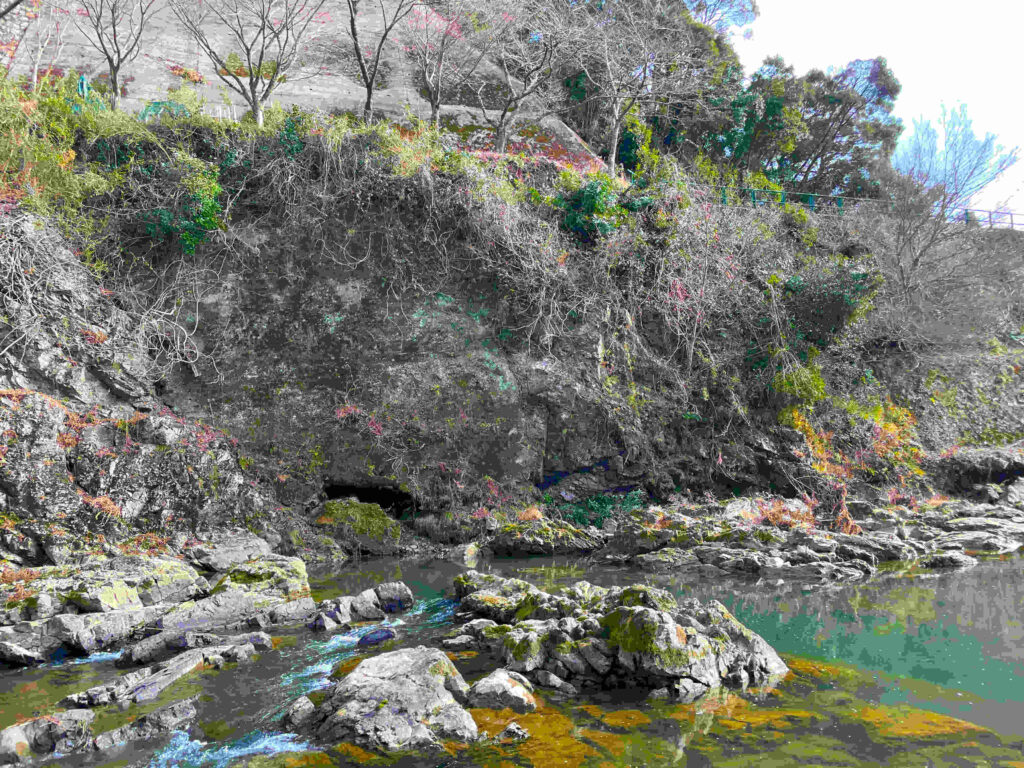
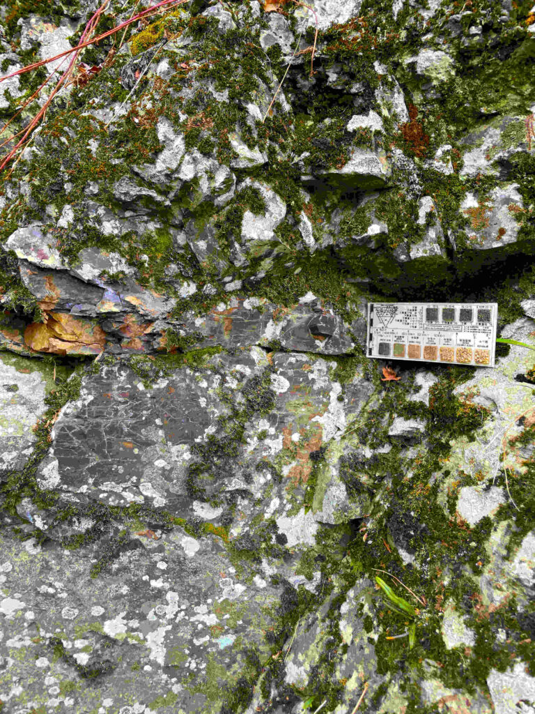
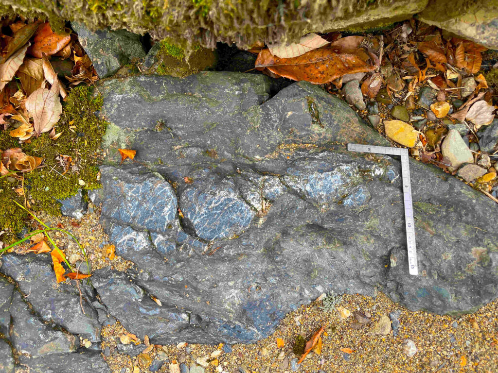
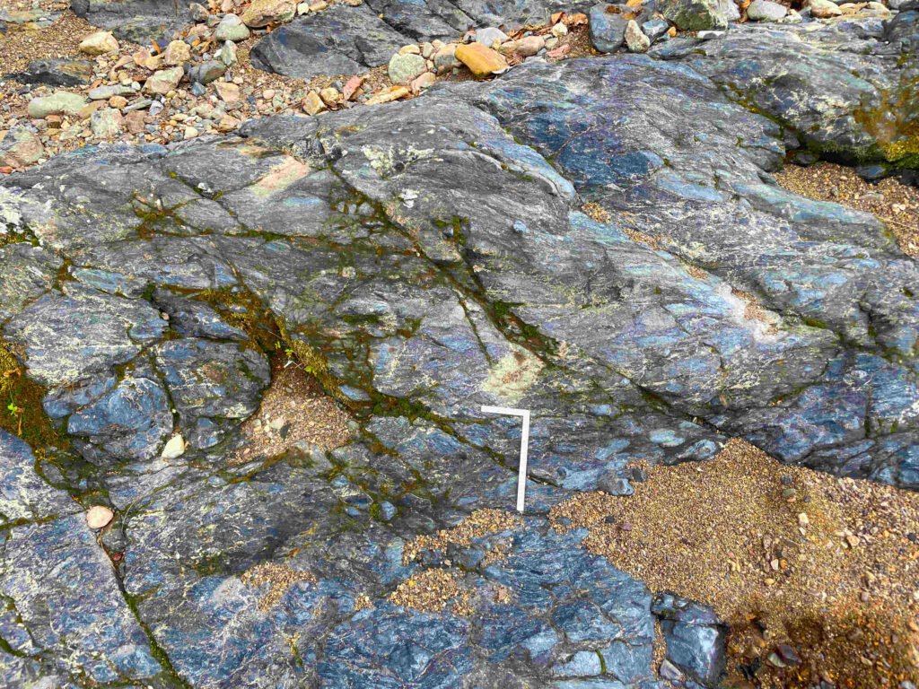
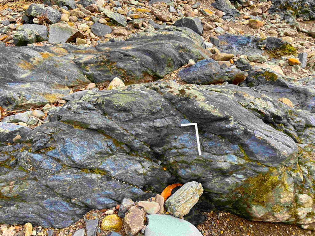
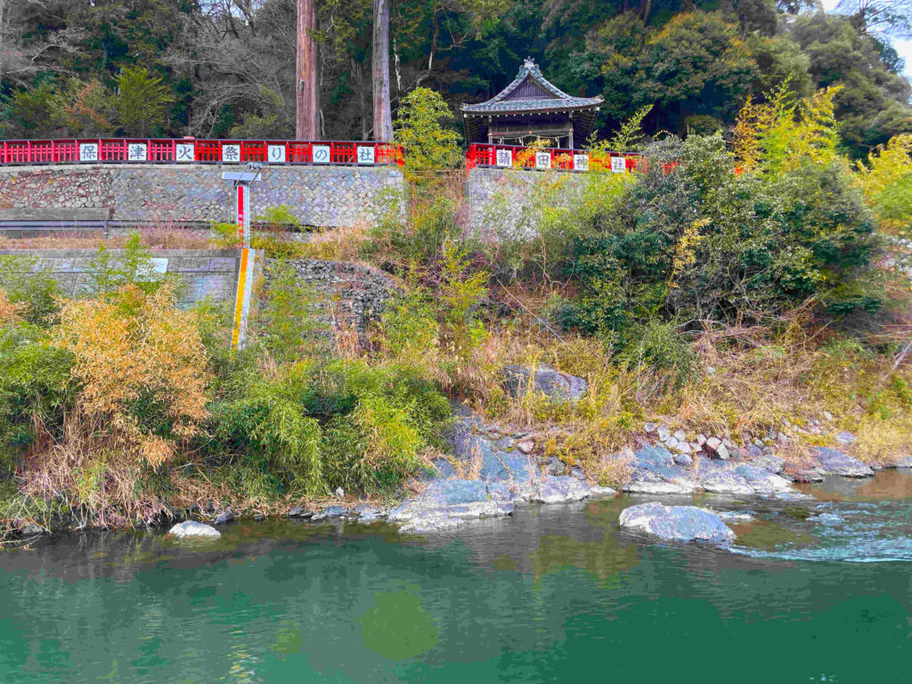
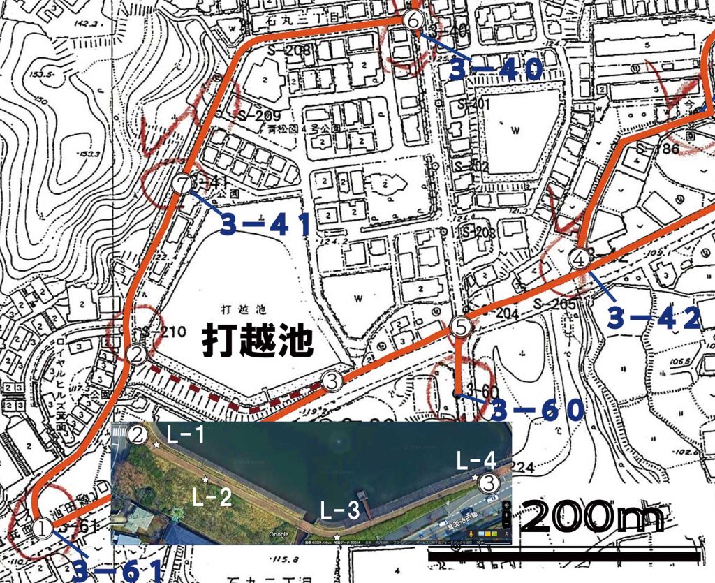
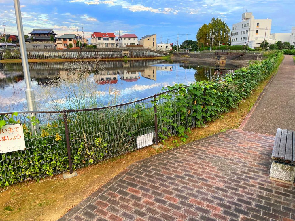
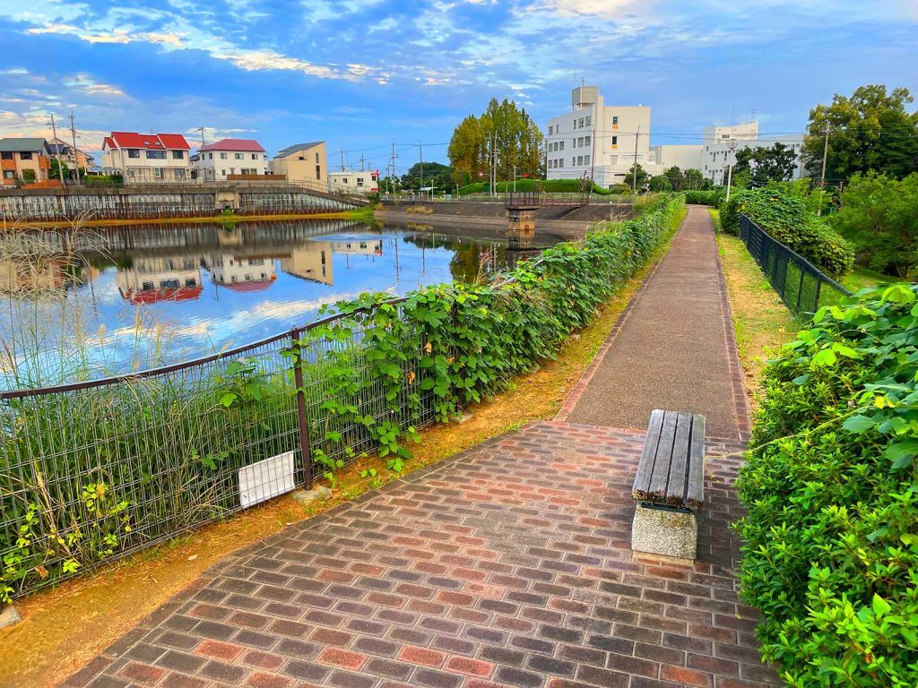
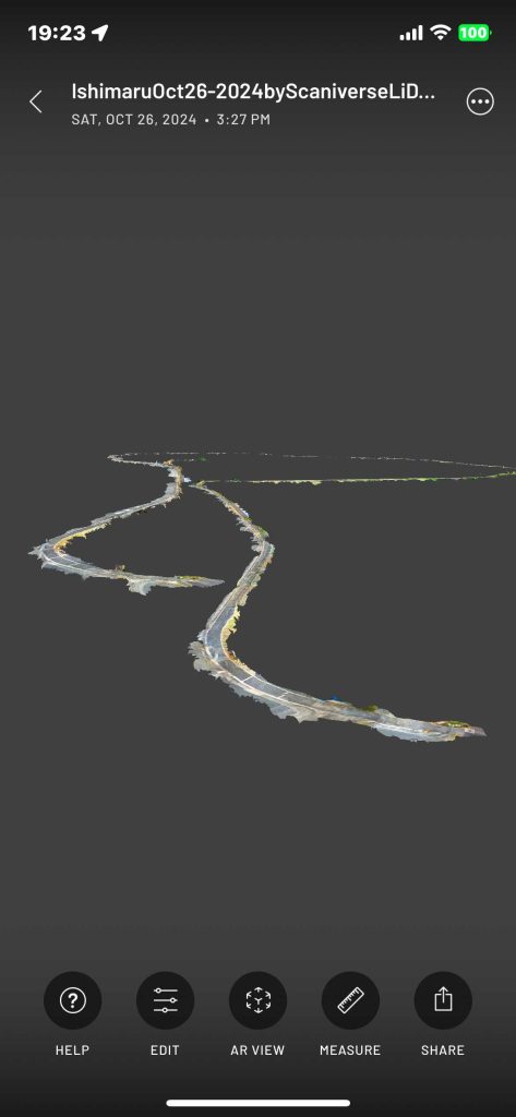
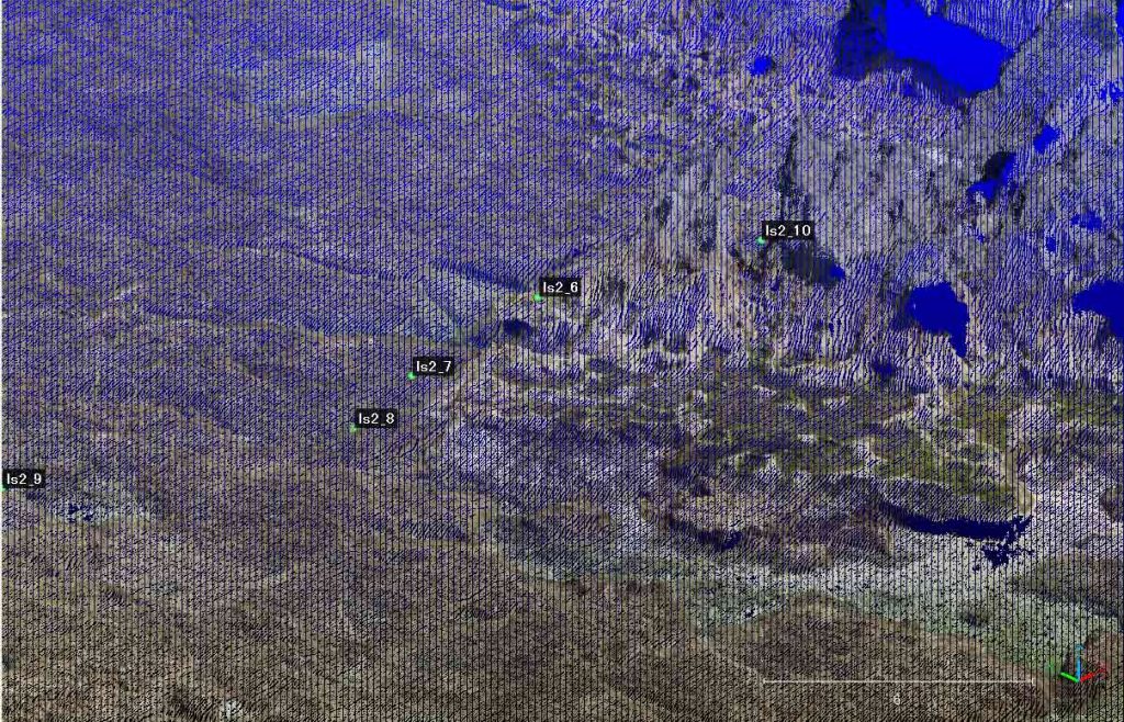
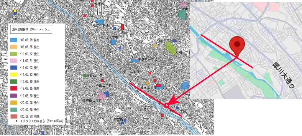
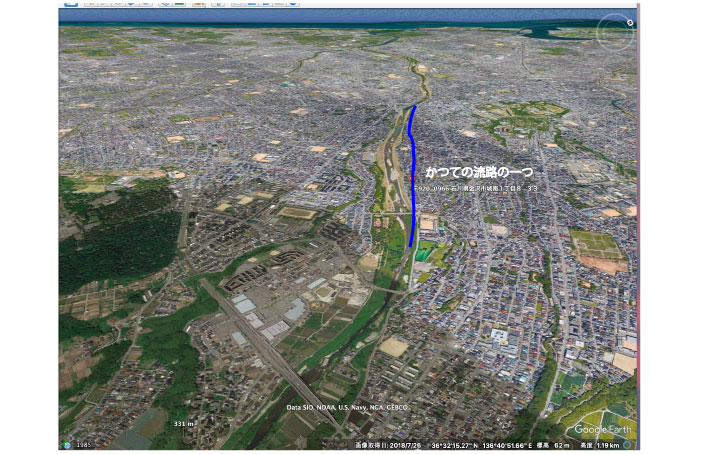
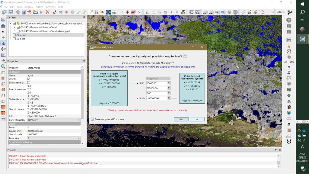
「古代タニハ『丹の海』とその排水プラグを地形発達史から復元 Part 1」関西大学文学論集75-4は本日(2026年3月12日)刊行されたが,この報告では,大山咋命が見た丹の海の湖面の海抜高度が98mであったことを明らかにした。図1の付近は海抜80mだからおよそ落差20mの滝があったとぼくは考えていた。その滝を数十年またはそれ以上の年数をかけて,開削をすることで,湖底は侵食されていったと想像したのである。開削工事については,上記論文のPart 2として発表する予定である。
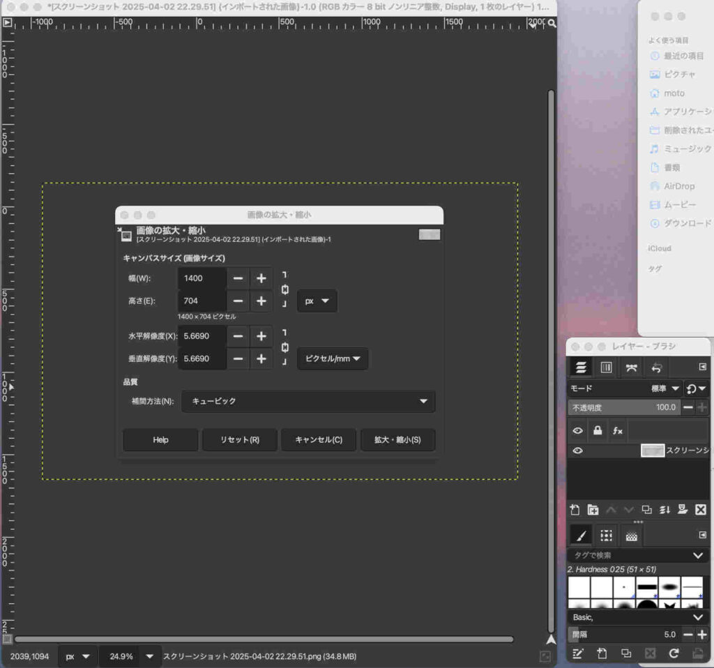
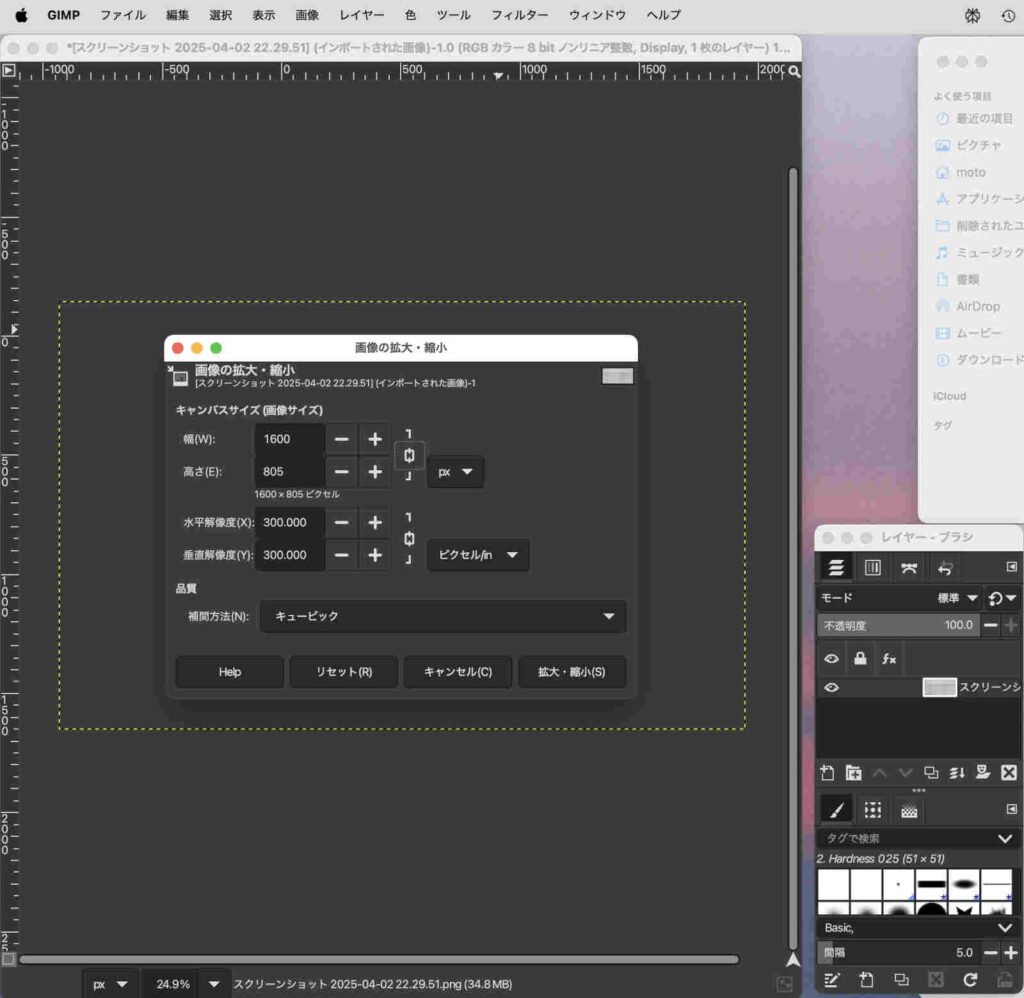
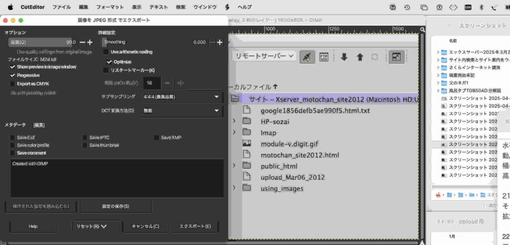
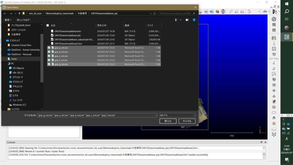
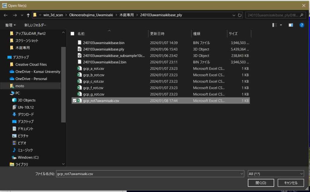
目的のファイルをダブルクリックすると選択できる。ファイルを選択したあとに右下隅の「開く」ボタンをタップしてもよい。 次に,Keep the image’s color profileパネルが表示される。この下端には「維持」と「Convert」ボタンがあり,「維持」ボタンをタップすることになる。ただ,このパネルは,「次回から確認しない」に☑️を入れて良いだろう。ぼくの能力では,このパネルを生かすことはできない。
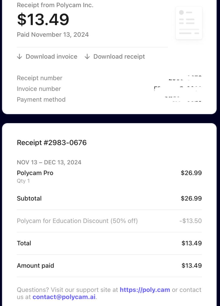
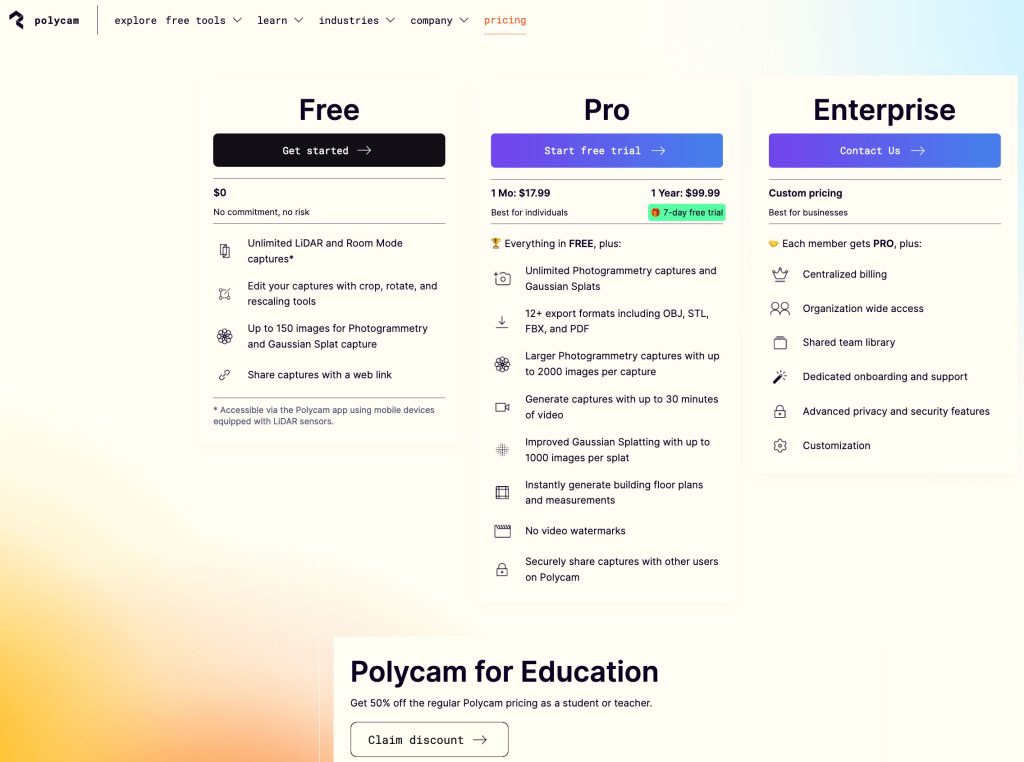
Please return ¥3300 = $26.99 per month for Polycam Pro to me. My apple account: xxxxx@xxxxx.ac.xxxx ————————————————
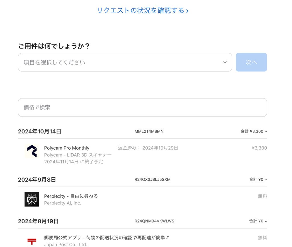
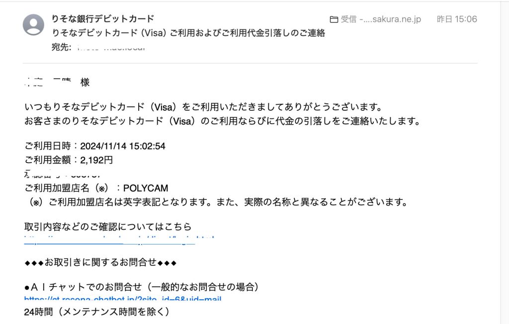
I bought “Polycam for Education” using my Debit Card you need on Oct. 14, 2024. “¥2103=$13.5 on Oct. 14, 2024” is shown in the Description of a trade of my city bank.
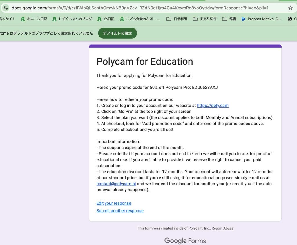
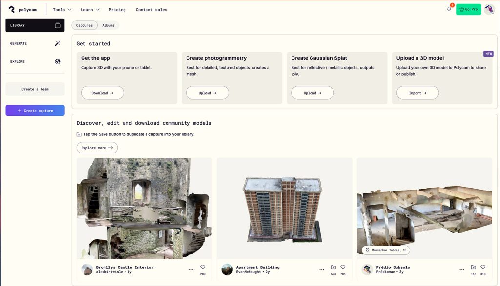
I had received your message: Polycam for Education Thank you for applying for Polycam for Education! Here’s your promo code for 50% off Polycam Pro: EDU0523AXJ Here’s how to redeem your promo code: Create or log in to your account on our website at https://poly.cam
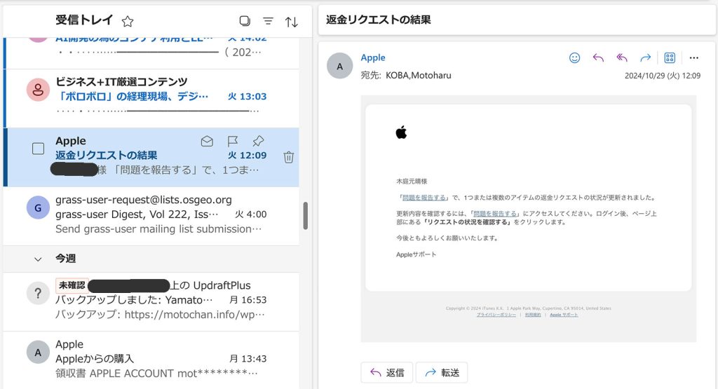
I recognized the following supposedly impermissible thing yesterday.
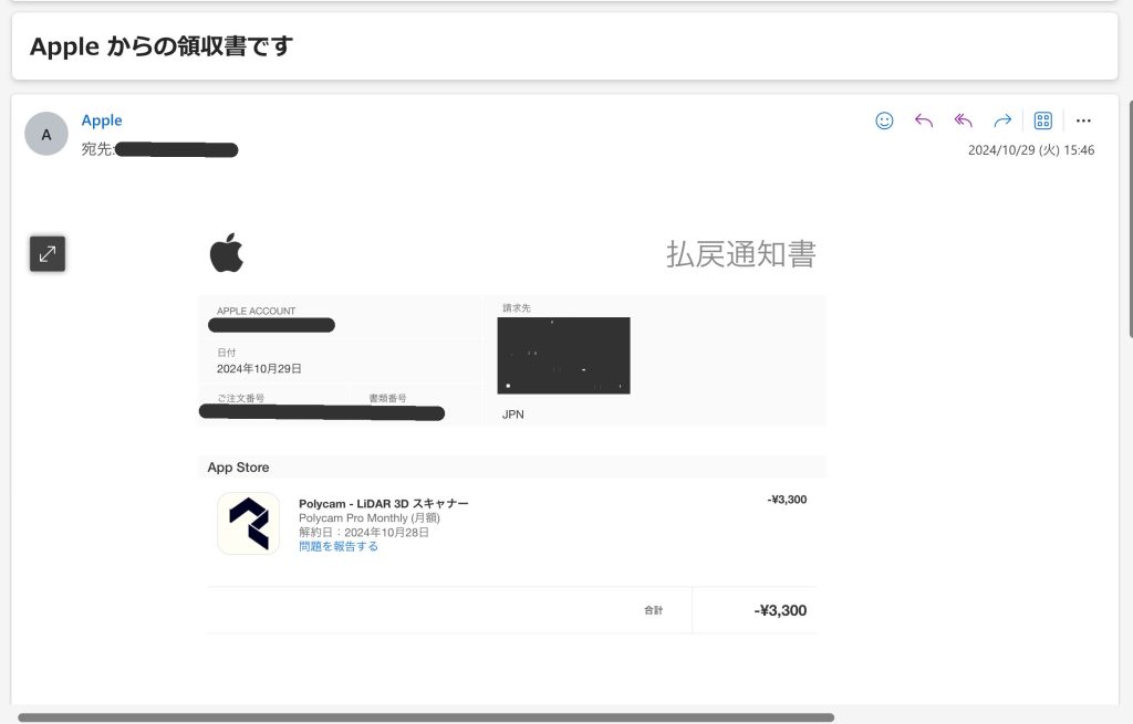
a. I found a mail from Apple Inc. to moto@kansai-u.ac.jp: a receipt of ¥3300 = $26.99 per month for Polycam _ LiDAR 3D scanner (order no: MML2T4M8MN)
b. I checked the billing details of my credit VISA card and found ¥3300 = $26.99 from Apple Com Bill.
———————————————— I made a phone call to the Apple Care, and advised to call you. Thank you. Oct. 28, 2024.
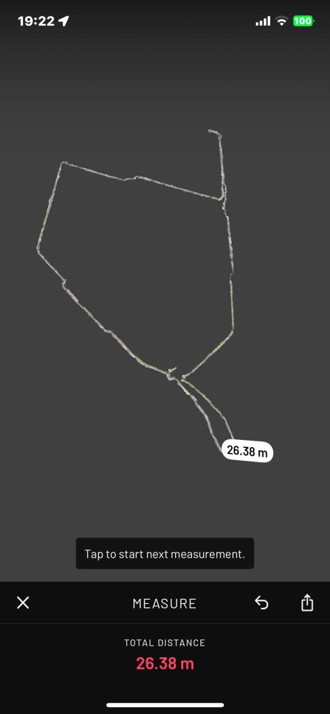
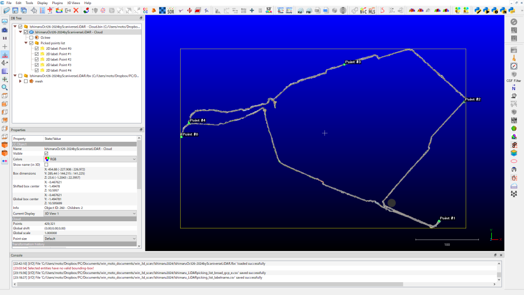
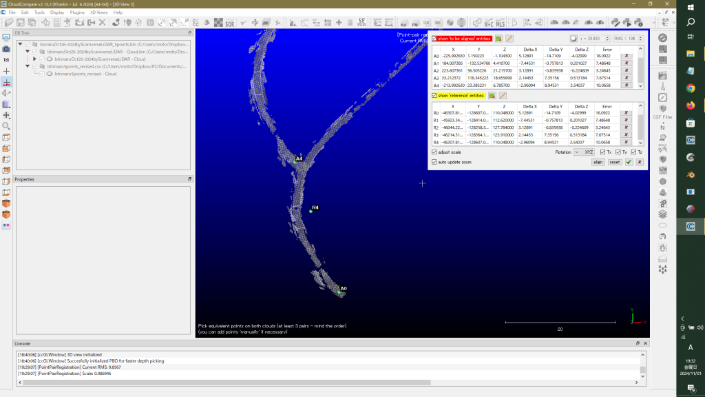
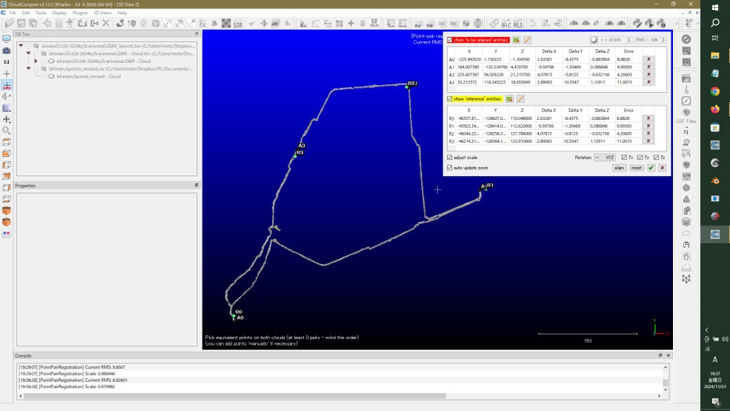
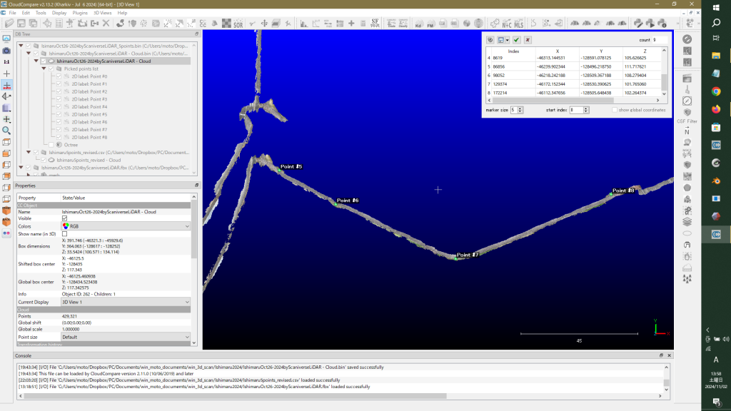
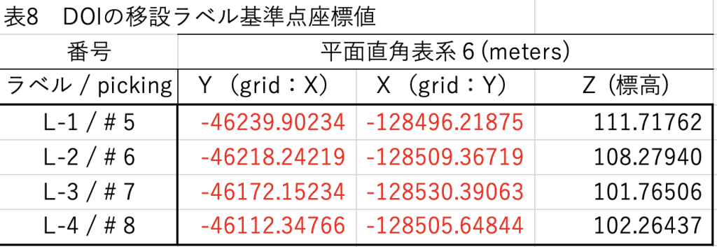
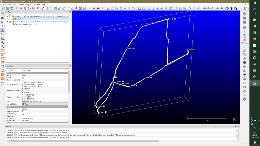
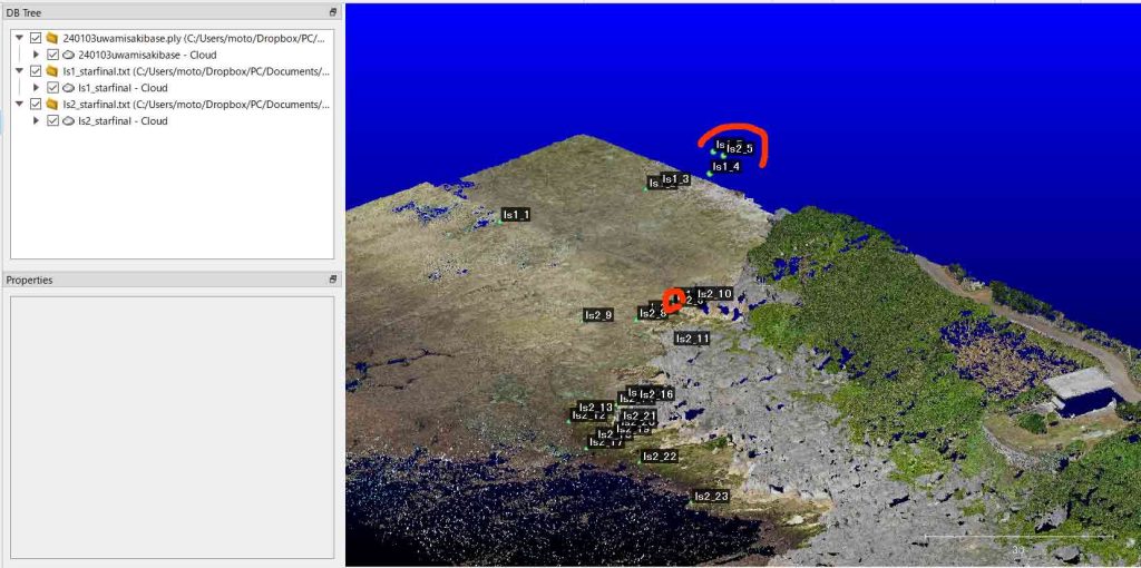
結局,ルート測量はLiDAR測量に限定されるということらしい。写真測量はかなりの情報が必要なのに比べて,LiDAR測量は,直接ベクトル長や方向角を捉えるために,空間把握が「高速」なのである。図1ではルート途中に打越池南縁のROIが含まれるのであるが,ルート測量の途中なので,このROI部分を詳細にスキャンするという発想もあったが,それは誤りである。ルートスキャン測量と詳細スキャン測量は別に考えた方がよい。前者で公共の基準点4点とROI内のLabels 1 to 4をスキャンして,公共の基準点4点からROI内のLabels 1 to 4の座標点を求めて,その上で,Labels 1 to 4を含むROI内の詳細スキャンを実施するのが適当ということになる。
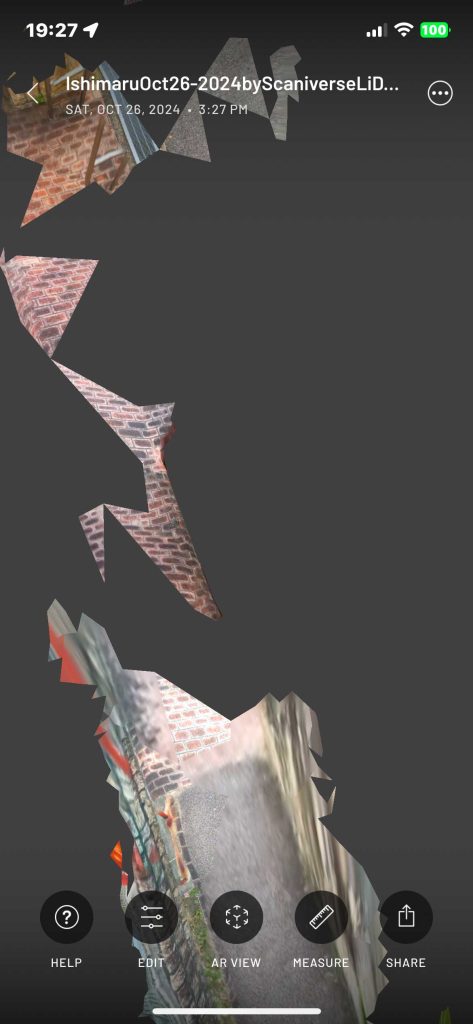
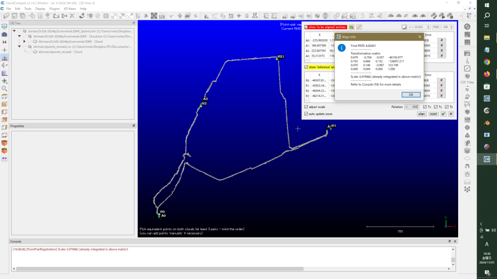
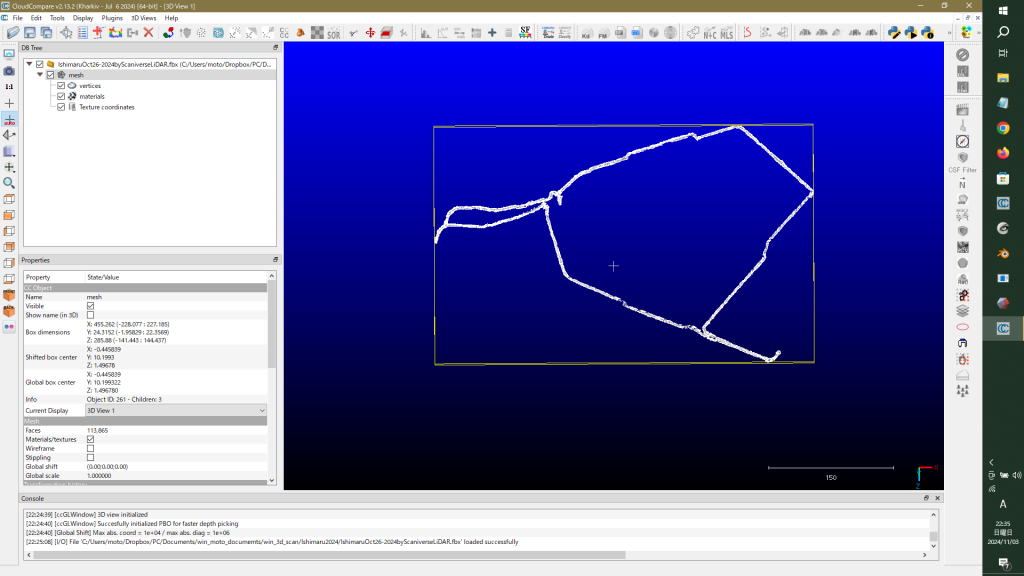
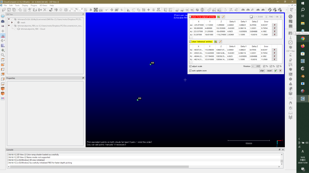
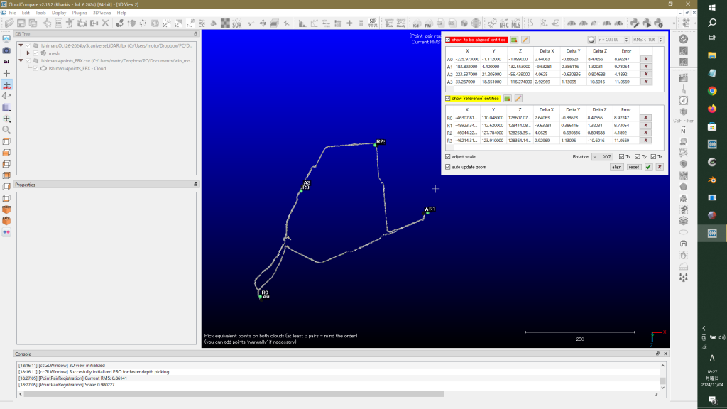
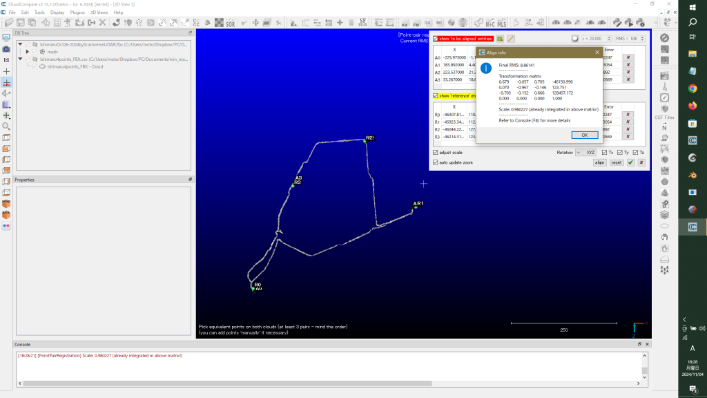
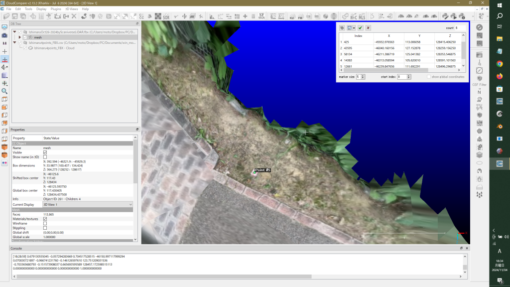
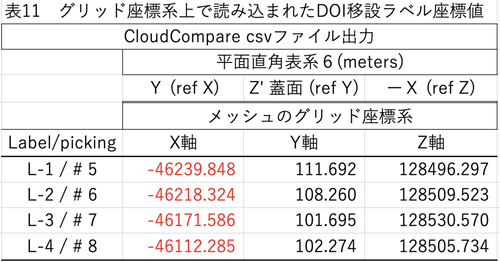
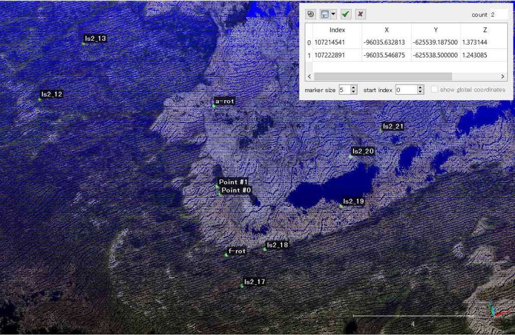
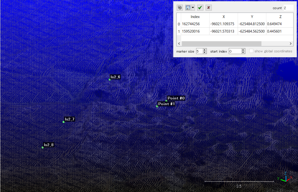
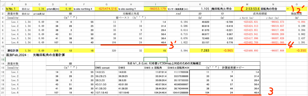
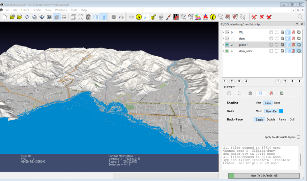
点群の平面図(Set top view)は,測量を実施した場の平面図と一致しているが,メッシュでは正面図(Set front view)の裏返し 3D image flipping が点群の平面図と対応している。そのため,pickingして表示される座標値は,(X, Z, -Y)になっており,基準点座標との関係を求める場合,注意が必要だと思うが,挑戦して,さいわい成功した。
以上,2024年11月2日。
7.1 メッシュと点群の座標軸の違い
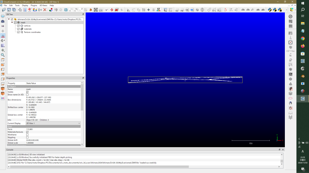
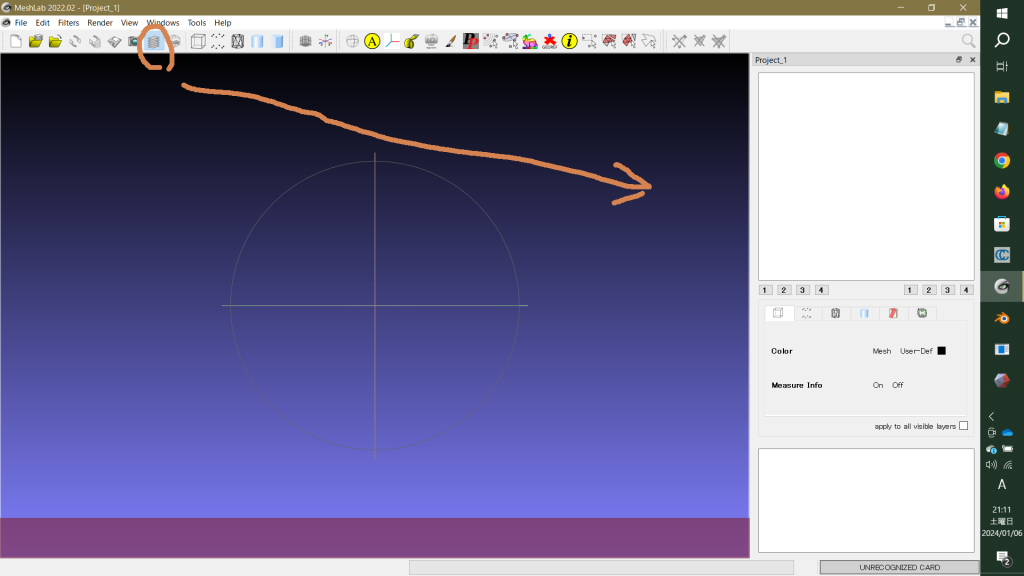
点群は感覚的によく合っているが,メッシュは開いたところがSet top viewにあたっているが,正面図だ。
図EE ScrnS 816
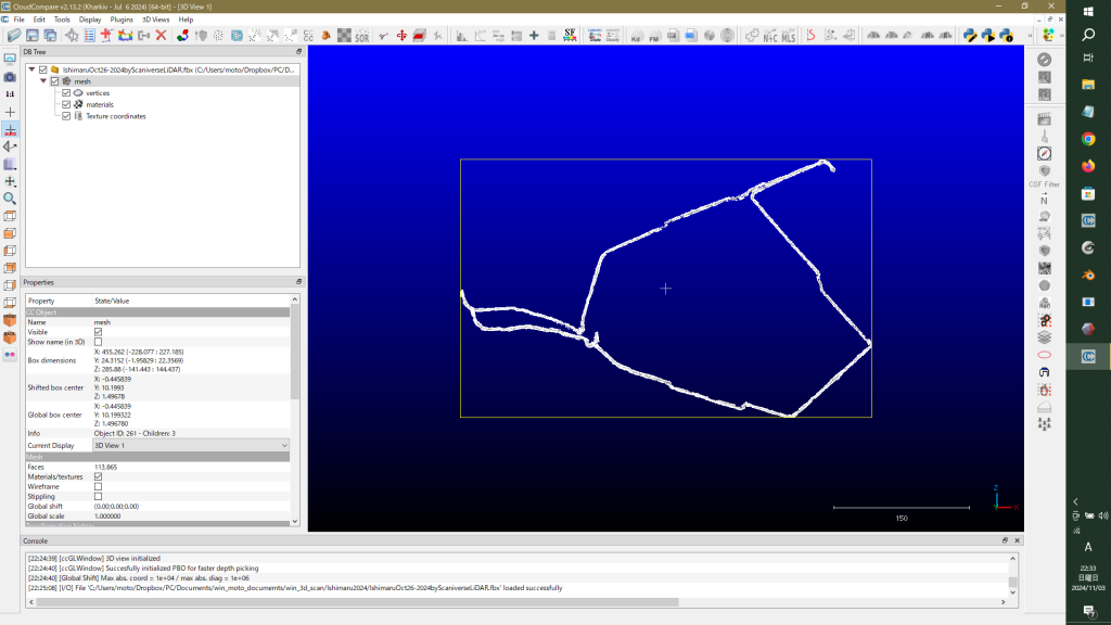
Set top viewにすると,図FFのように,平面図になる。
図FF ScrnS 817
裏返したのが図GG。右下の座標軸を見ると,水平右方向がX,水平下方向がZ,そして垂直方向がYだ。
図GG ScrnS 818
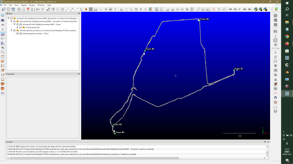
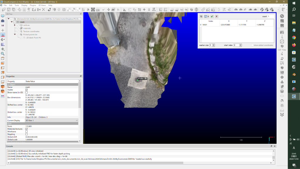
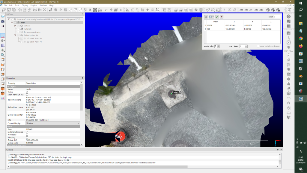
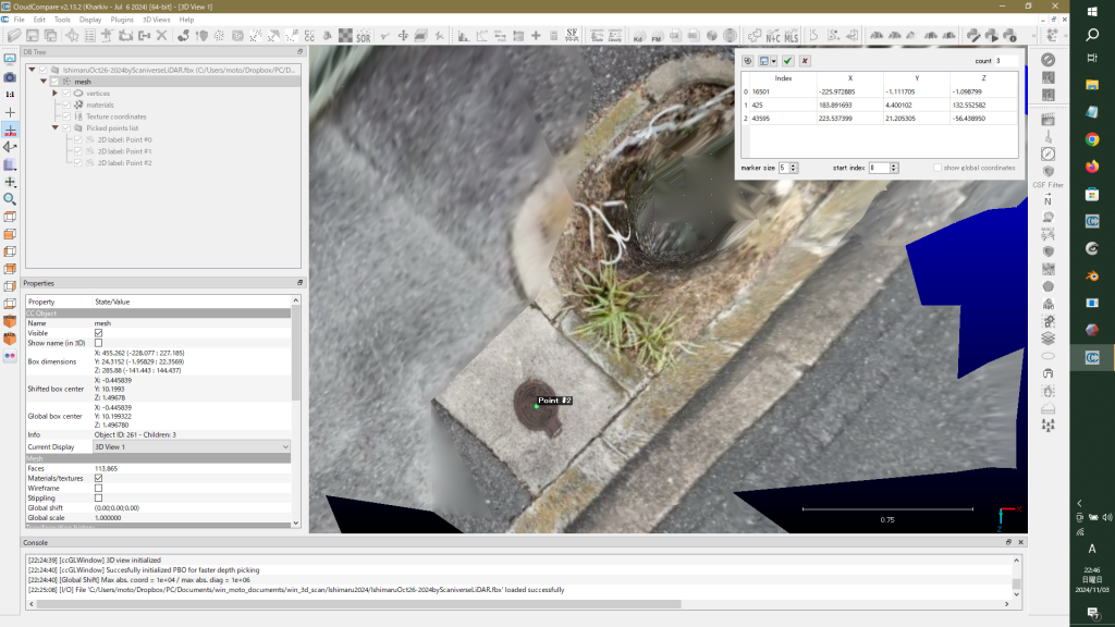
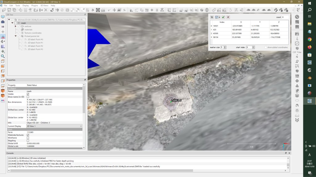
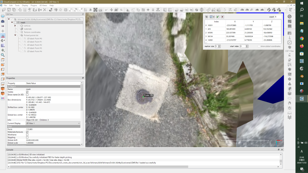
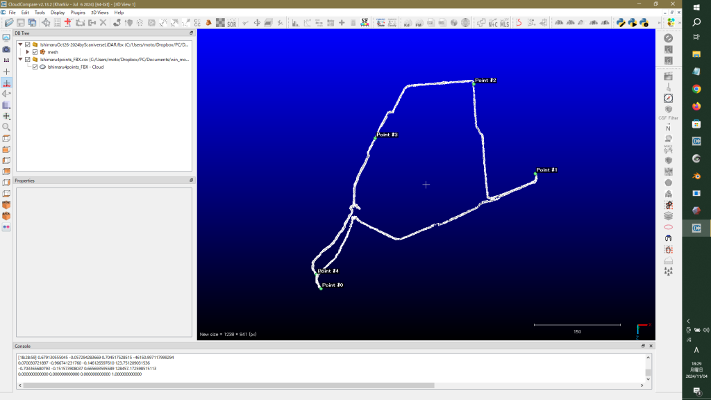
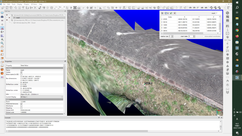
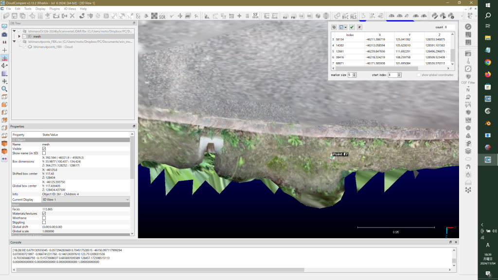
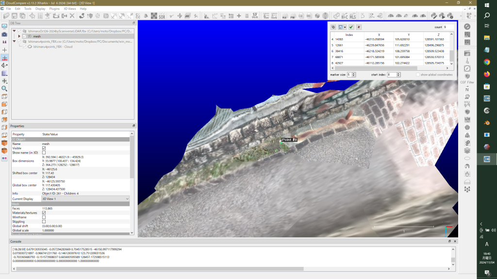
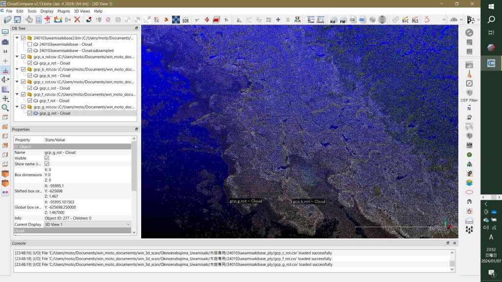
点群とメッシュの比較をするために,図Aの各基準点対応のメッシュ座標値をPoint List Pickingしてみよう。Point #1 to #4だ。図Aの,①,④,⑥,⑦,①だ。図819〜823を見ると,ハンドホールがはっきりと見える。点群と全然ちがう。
図819 ①
図820 ④
図821 ⑥
図822 ⑦
図823 ①’
7.2 メッシュ上でのPoint List Picking
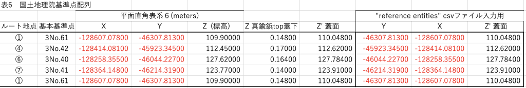
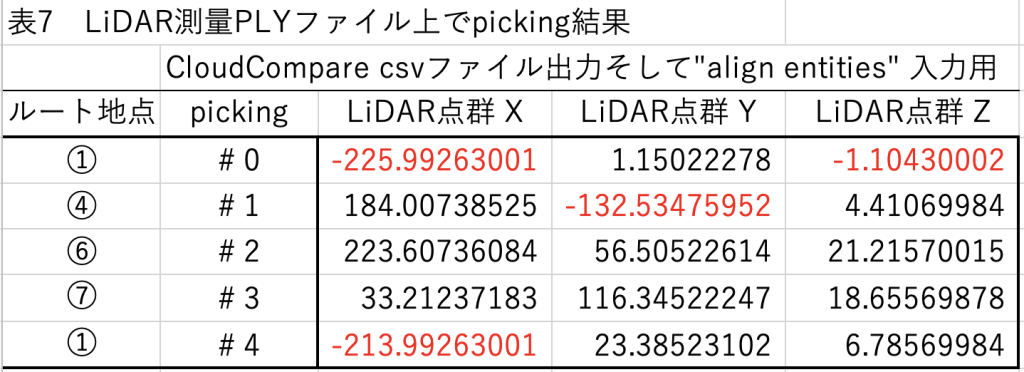
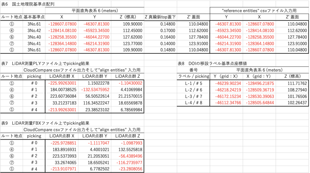
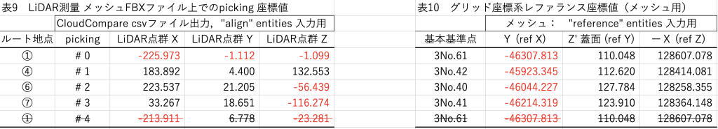
Point List Pickingの結果はcsvで出力した。その結果を表9に示すが,前述のように,点群 (Y, X, Z’)は,メッシュ (Y, Z’, -X) になっている。鬱陶しいだろうが,表6も追加したものを次に。
洞窟測量におけるPolycam(3Dスキャンアプリ)操作マニュアル 関連の書誌は次のよう。 小竹祥太,林田敦,柏木健司,2023. iPhone Pro によるLiDAR 測量を活用した洞窟調査: 七久保の道穴(群馬県下仁田町青倉川上流)を例として.群馬県立自然史博物館研究報告, No. 27, pp. 171-179. Kotake, S., Hayashida, A. and Kashiwagi, K., 2023. Cave survey using LiDAR measurements with the iPhone Pro: an example of Nanakubo-no-michiana Cave(limestone cave)in the upper reach of Aokura River, Gunma Prefecture of central Japan. Bull. Gunma Mus. Nat.Hist., No. 27, pp. 171-179.
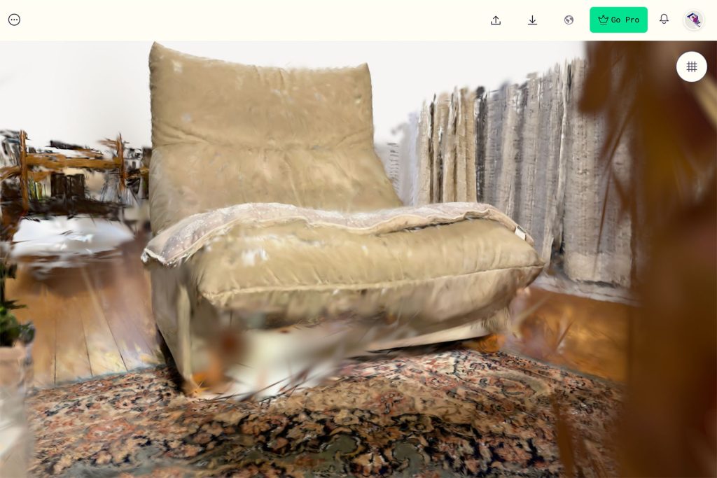
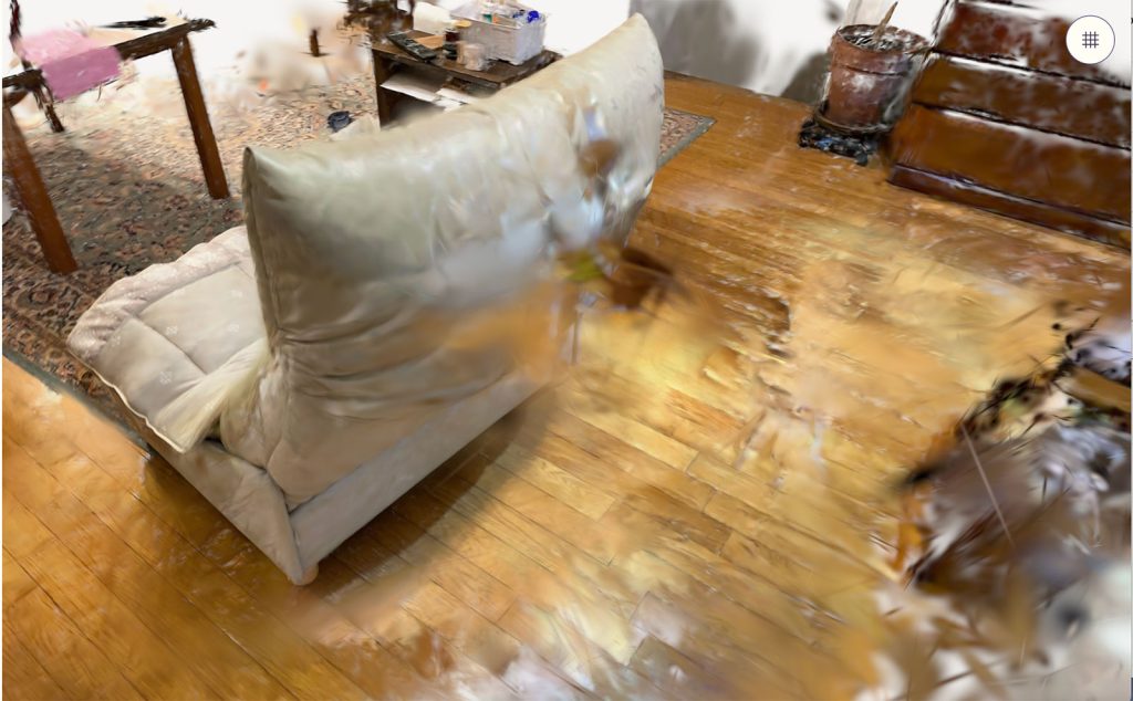
1 iPhone Pro によるLiDAR 測量を活用した洞窟調査: 七久保の道穴(群馬県下仁田町青倉川上流)を例として—————— これを見ると,iPhone ProのLiDAR測量は便利やなあ,という感想,ということで,ぼくの体験や感想も同じだ。 p. 172右段の方法,では,「iPhoneに搭載されたLiDARは,搭載カメラが撮像可能な明るさ環境で,スキャン対象の色情報の取得が可能である.洞窟記載の基礎データとなる洞内測図を作成するため,洞内ではiPhoneにヘッドライトを固定してLiDAR測量を実施した」とあった。「色情報の取得」というか,明るくないとLiDAR測量はできない。 p. 174左段では,「LiDAR測量に要した時間は事前の下見を含み約15分であった.七久保の道穴周辺の地形断面の概略を把握するため,沢床から町道,洞口,および洞口上方の尾根まで,LiDAR測量を分割して実施した.全体を先ずは見渡し小崩壊地形を避けてルートを設定し,沢床から斜面を傾斜方向に登りながら測量した」,とあって,洞穴外の地形もLiDAR測量されている。ぼくもこの種の作業を実施したが,iPhoneのLiDAR測量能力は凄い。 p. 177の議論では,「iPhoneを利用したLiDAR測量は,iPhoneそのものが小型かつ片手で操作が可能であり,狭い空間を含む洞窟での測量において高い利便性を有する.一方,LiDAR測量に伴うiPhoneのバッテリーの消耗は大きく,複数の洞窟を対象とした筆者らのこれまでの試行では,3-4時間程度でバッテリーが低レベルの状態となった.考えうる現時点でのバッテリー対策としては,予備のモバイルバッテリーの準備,ないし車が近くにある場合はシガーソケットからの充電などが考えられる.また,複数名でLiDAR測量を行う場合,スキャンする空間を計画的に割り当てることで,一定規模の洞窟空間をカバーするLiDAR測量が可能である.計測範囲の5 mを越える平面的に広い空間については,洞床と洞壁を含みくまなく歩いてスキャンすることで,データ取得は可能である.一方,天井の高い空間については,自撮り棒や伸縮性ポールの先端にiPhoneを取り付け,長さと方向を調整しながらLiDAR測量を行うなどが想定できる」とある。まあバッテリーは安いので複数持参すれば問題はない。
補助的な測量や公共基準点からの位置づけなどがされているのではと思ったが,無かった。
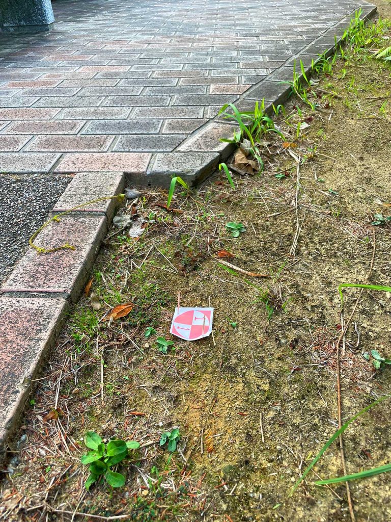
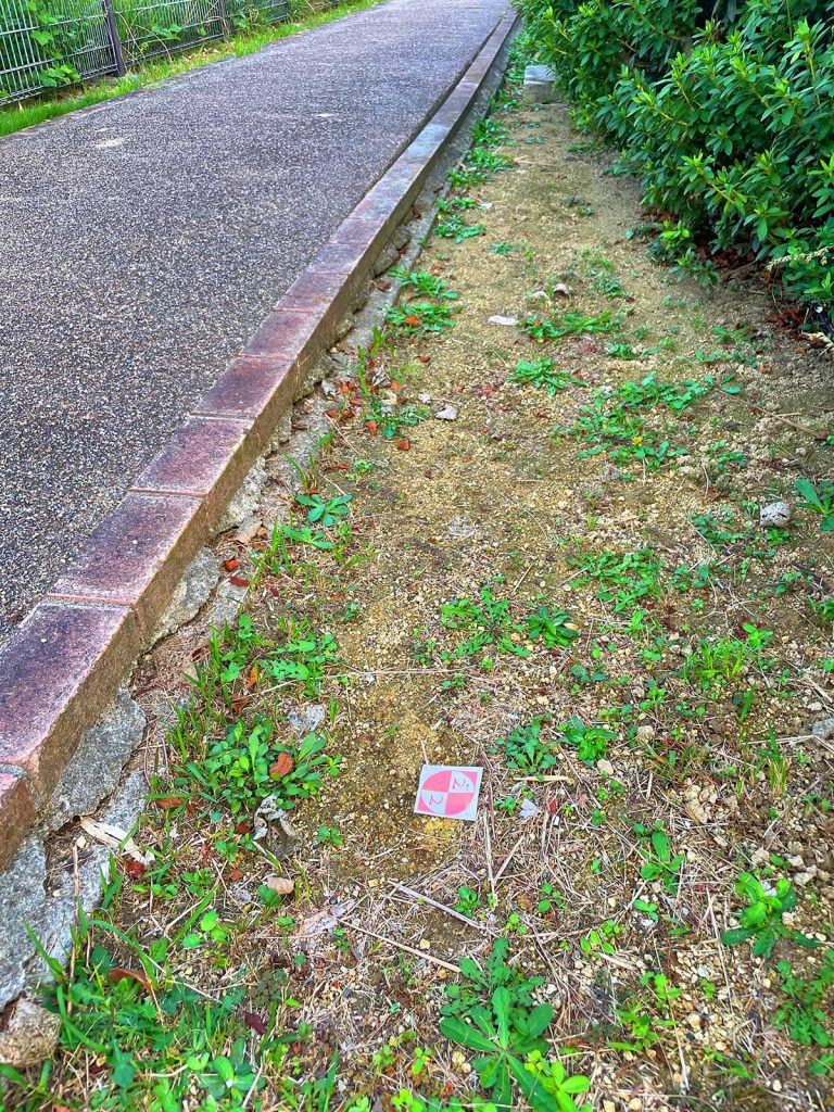
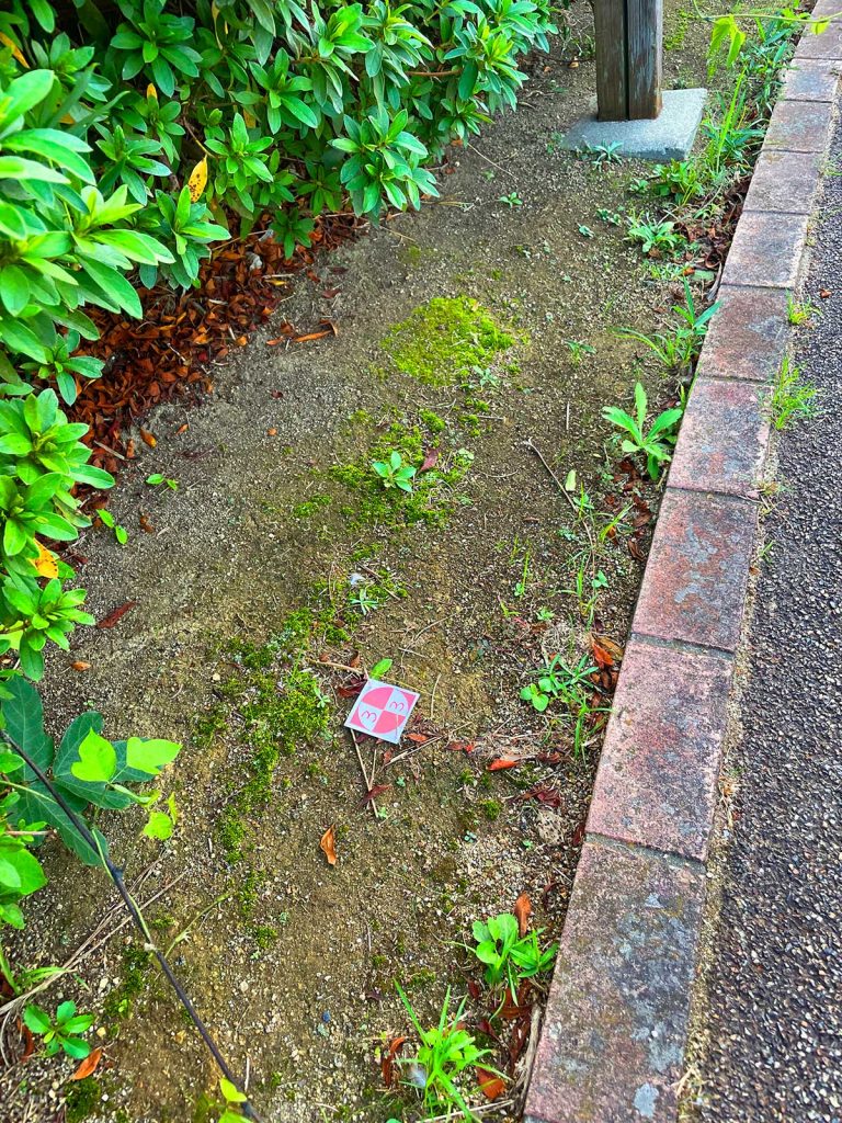
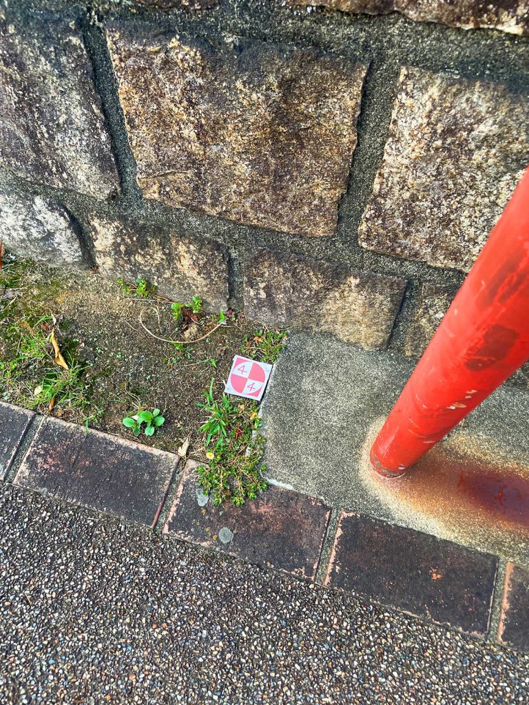
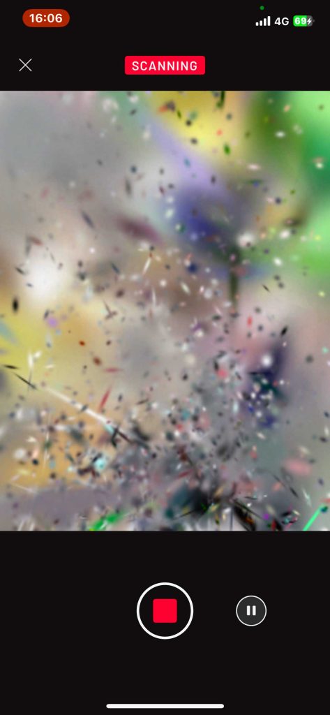
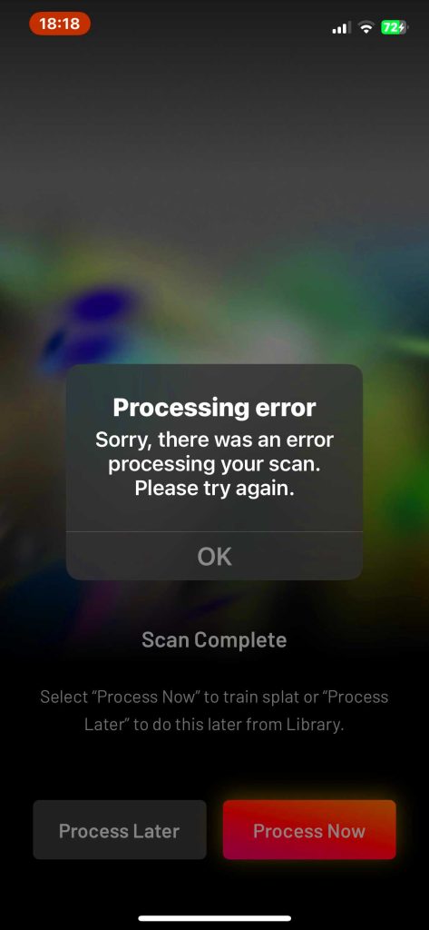
2 付ファイル01 洞窟測量におけるPolycam(3D スキャンアプリ)操作マニュアル—————— この報告にはページ番号が振られていない。 4枚目の,4.Polycam の応用的な使用方法,で,次の記述は参考になった。 「4.1 スキャンの一時停止および再開 Polycam のスキャンには一時停止機能がある.スキャン中を示す赤色の録画ボタンの右横の一時停止ボタン(図1 の④)をタップする.すると,画面下に「capture paused」が表示される.再開には「○に▷記号の入るアイコン」をタップし,終了時には赤い録画ボタンをタップする.一時停止機能は,狭洞など円滑な動きが難しい空間での測量に効果的で,一時停止後にスキャンし易い体制に体を入れ替え,スキャンを再開する. Polycam には,スキャン終了後にスキャンを再開できる機能がある.再開する場所ないし対象物付近で過去のスキャンデータを開き,画面下部の「追加」アイコンをタップする.「追加」アイコンが見当たらない場合は,画面下を左右にタップしてアイコンを移動させる.過去にスキャンした3D データとスキャン中の3D 形状に,相互にオーバーラップする形状が認識されると,「relocalization successful! You can now proceed to scanning new areas」と表示され,白い録画ボタンを押すとスキャンが再開される(図1 の⑩).洞窟の分岐に加え,スキャンし忘れた箇所の補完に対応できる.なお,「追加」機能はデータサイズの増加につながり,ファイルサイズが大きくなることでアプリのエラーや強制終了が生じることがある.また,過去の3D データにオーバーラップする範囲が認識されない場合,「rescan the place you originally scanned to extend, targeting visually rich areas」として「iPhone を動かして開始」という表示が画面上に示される(図1 の⑪).我々の数度の経験では,同じ場所のスキャン再開は問題なくできたので,iPhone を様々な方向に動かしてもこの表示が消えない(再開に移行しない)場合は,スキャン対象である場所ないし対象物を間違っているか,同じ場所であっても改変が生じた可能性を考慮する必要がある. 4.2 スキャンの分割 一度にスキャンする空間の大きさやそれに伴うデータ量に依っては,取得データのサイズが大きくなり過ぎることでPolycam の処理にエラーが発生し,またはPolycam が強制終了することがある.どの程度の広さや長さを目安に,スキャンする空間を分割するのが適切ないし最適であるかは,調査目的に係 るスキャンの精度に紐付けされる取得データ量に左右され,数字で示すことは難しい.なお,一定以上の空間を対象に分割してスキャンする際,後の3D モデル結合処理の際の利便性を考慮して,目安として2-3 m 程度の重複を必ず確保しておく必要がある.また,特徴的な形状が含まれる空間で重複を取ることが望ましい.メモ:この赤字化した部分だが,ぼくの場合,紙で作ったマーカー(四分割対角黒白塗)を貼っている。 4.3 データの再処理 Polycam では,処理済みの3D データを繰り返し処理できる機能が備わっている.処理済みの画面下に並ぶアイコンのうち,左端の「処理」をタップ(図1 の⑦)すると,処理画面に移動する(図1 の⑤).ここで右下の「カスタム」をタップすると,深度範囲,ボクセルサイズ,簡略化,自動クロップ,LOOP CLOSURE について,処理条件を調整できる(図1 の⑫).処理条件を調整後に「処理」をタップすると,画面中央のダイアログボックス内に「Reprocess capture? This will overwrite the existing capture and erase your edits.」と表示される.以前に処理した3D 画像データは上書きされるので注意が必要である.処理を続ける際は「はい」をタップする.すると,新しい条件での処理が開始される」
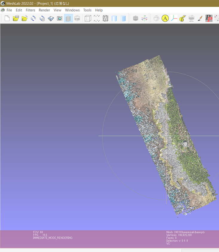
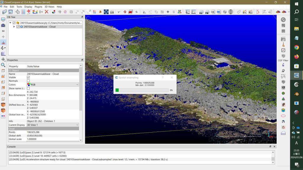
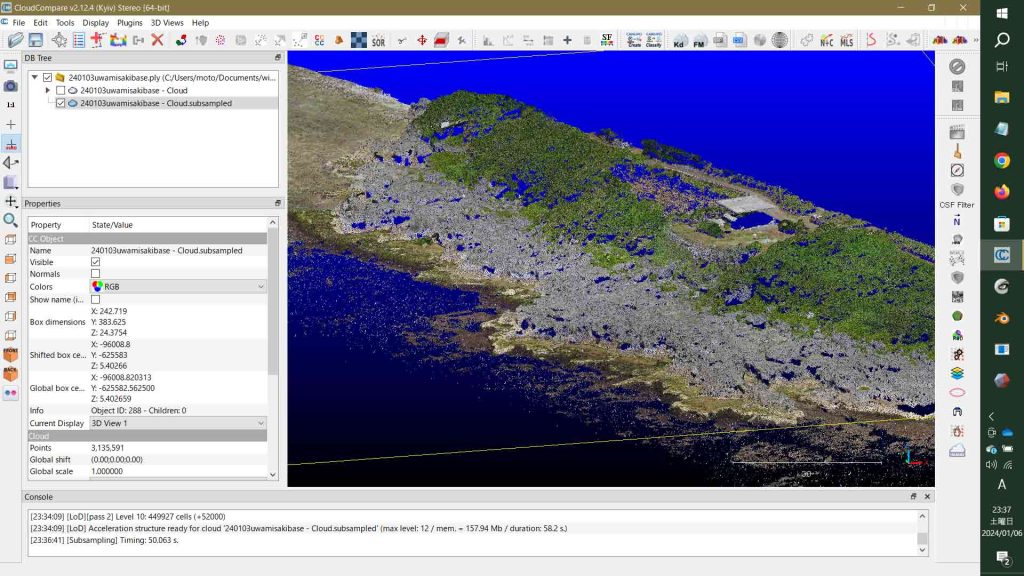
狭い範囲のdrone測量3Dmapをスムーズに観察できない。mouse製のGeforce(NVIDIA社が設計開発しているGraphics Processing Unit (GPU) のブランド名)を銘打っているゲームマシーンであるが。メモリは64GB,もう十年ほど前に購入したものだ。人生が残り少ないので,新たな投資はどうかと思うが,ちょっとネットでみた。
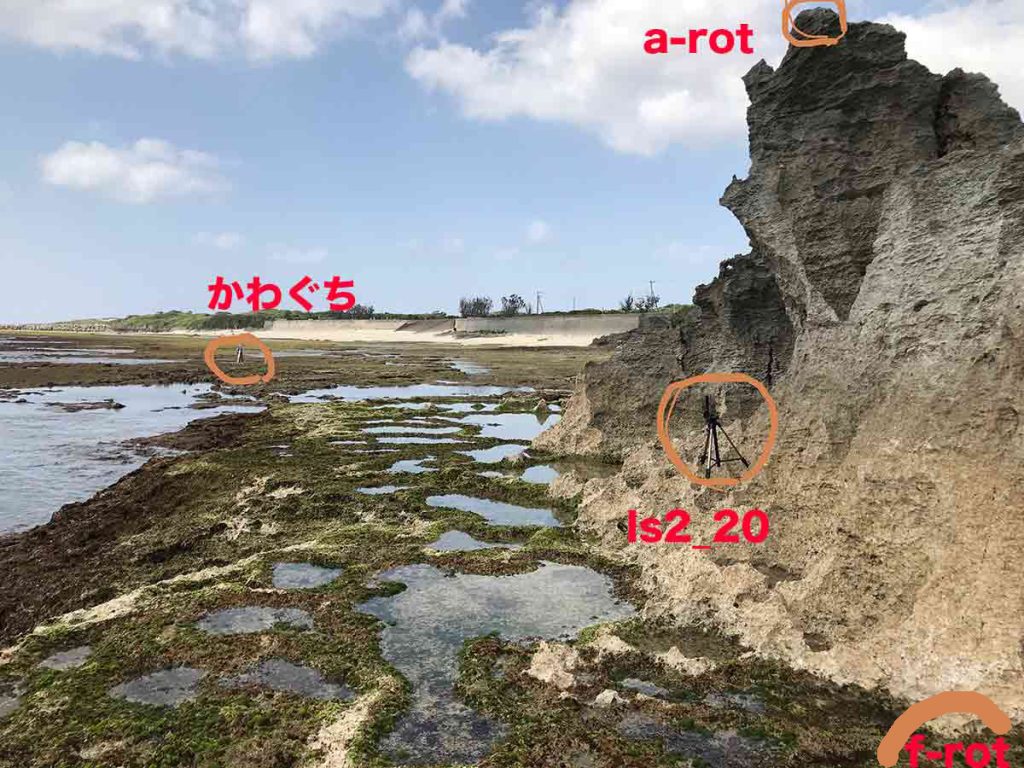
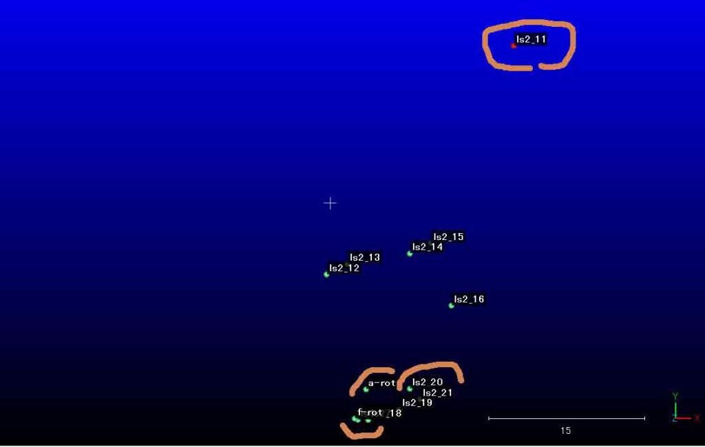
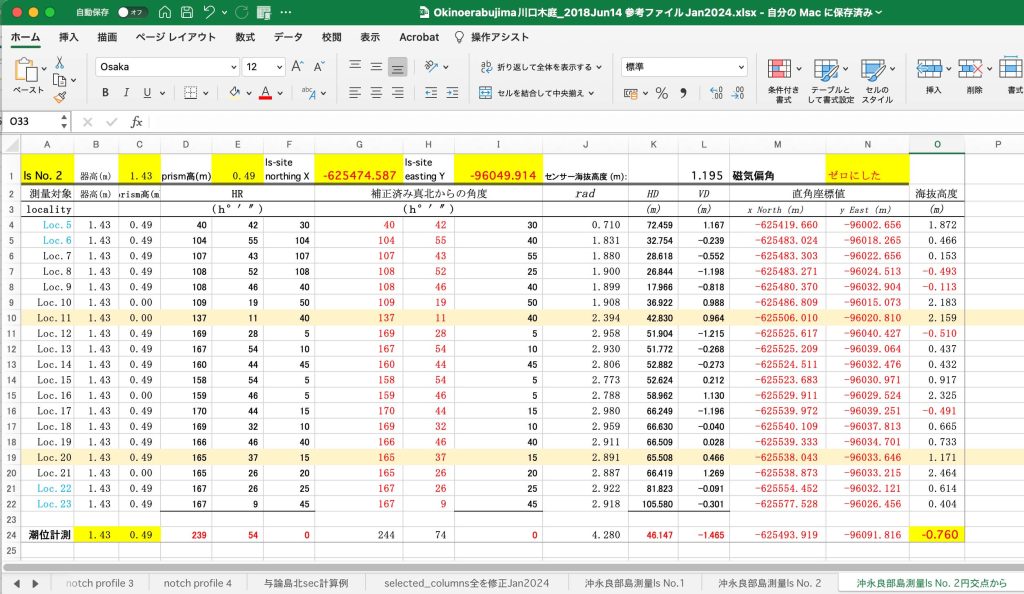
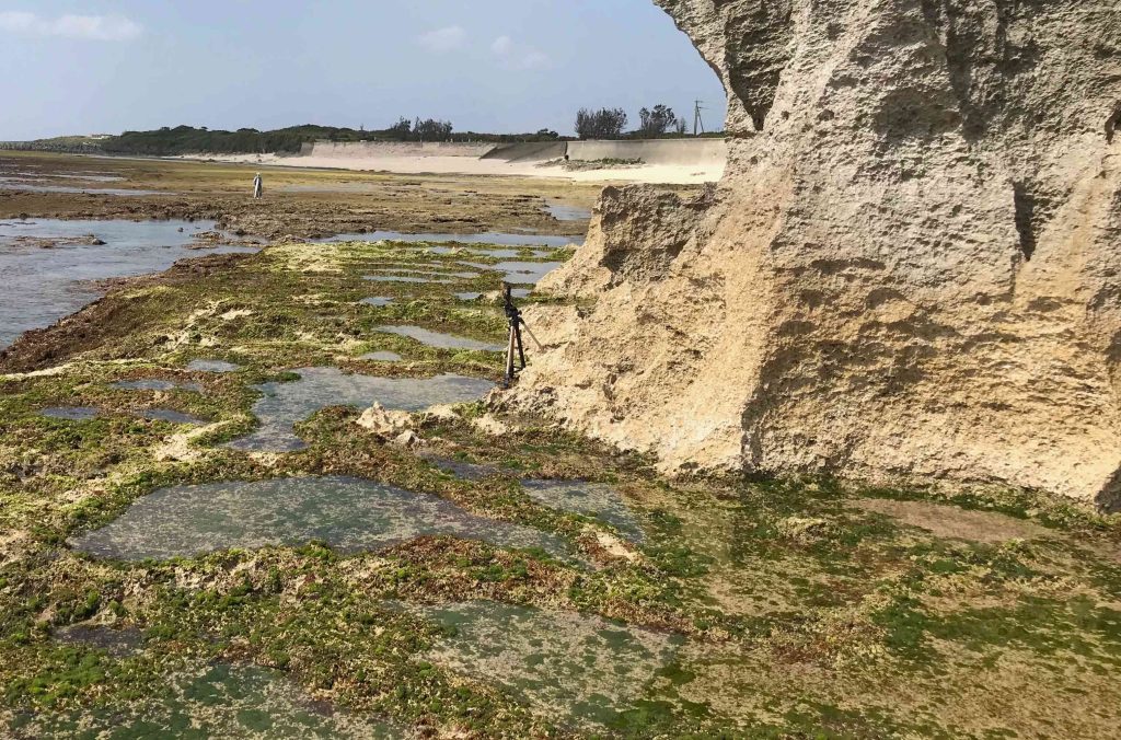
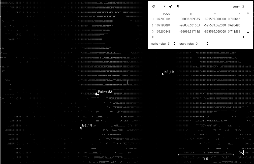
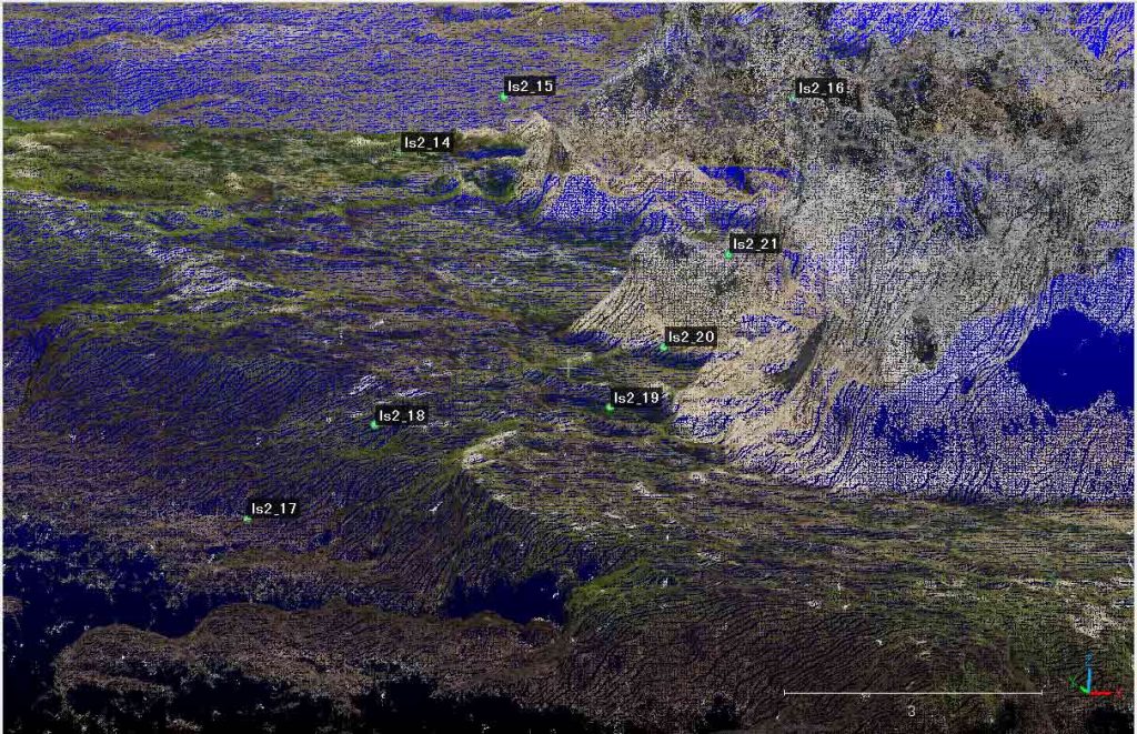
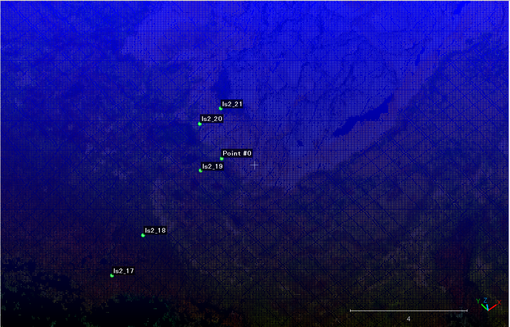
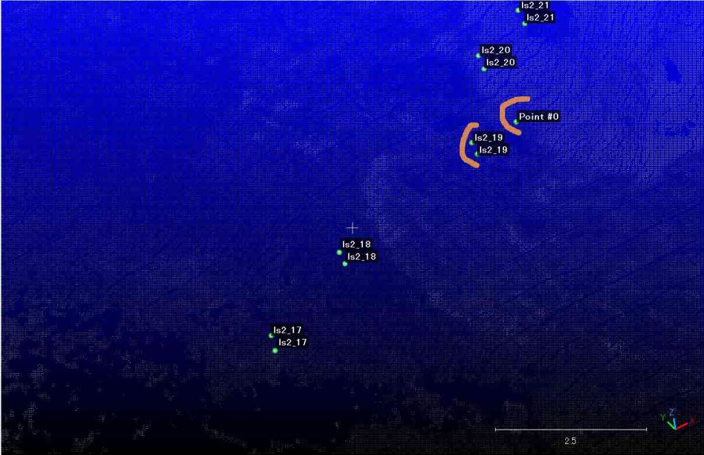
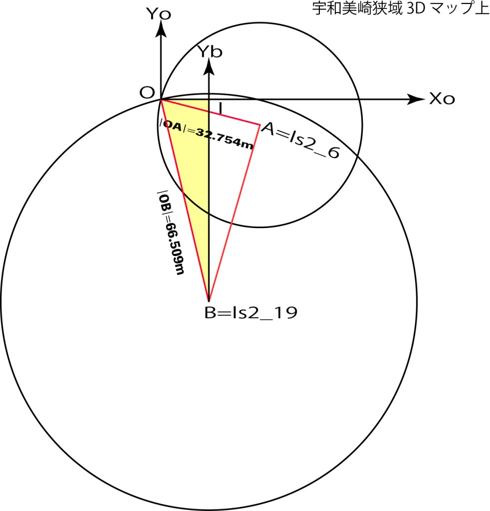
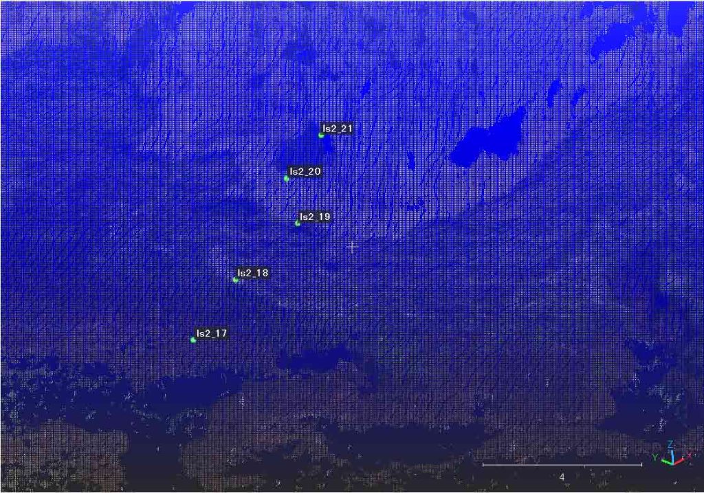
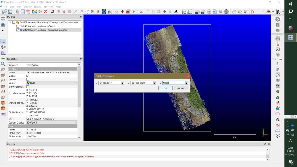
ls2_19の図10での想定位置位置を,図9の現場写真から決定した。図10の表の2の位置が適当と思われる。図10の鮮明度は低く,2階調にしている。このデータは次のようである。 X easting =-96036.617188, Y northing = -625539.000000, Z = 0.711838
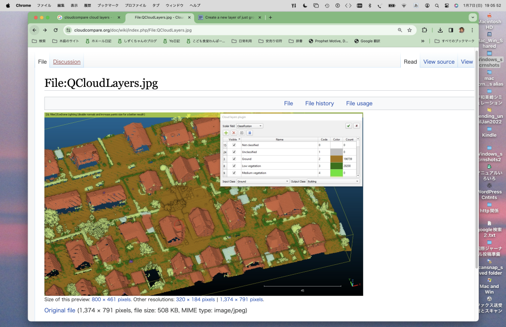
Danielさんが,フォーラムで, Maybe you can use the new ‘qCloudLayers’ plugin? Another way, maybe more simpler, is to use the ‘Edit > Scalar fields > Split cloud (integer values)’ method. This will create as many (sub) clouds as classes present in your cloud.
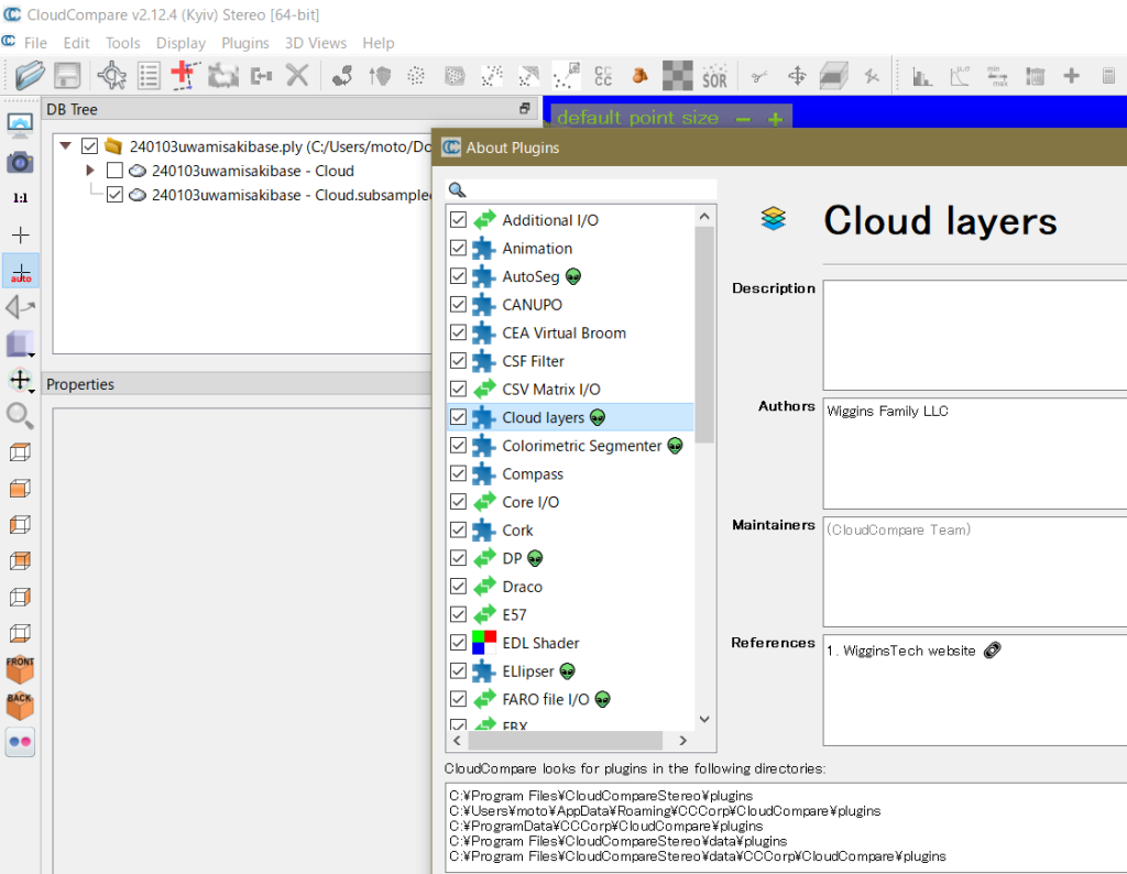
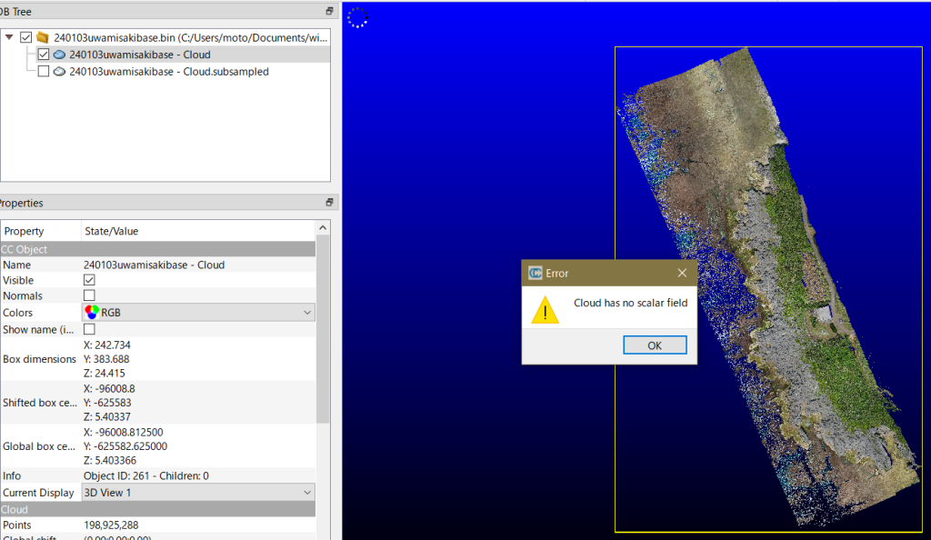
図6 Cloud layersを選択すると,Cloud has no scaler fieldsのエラーが
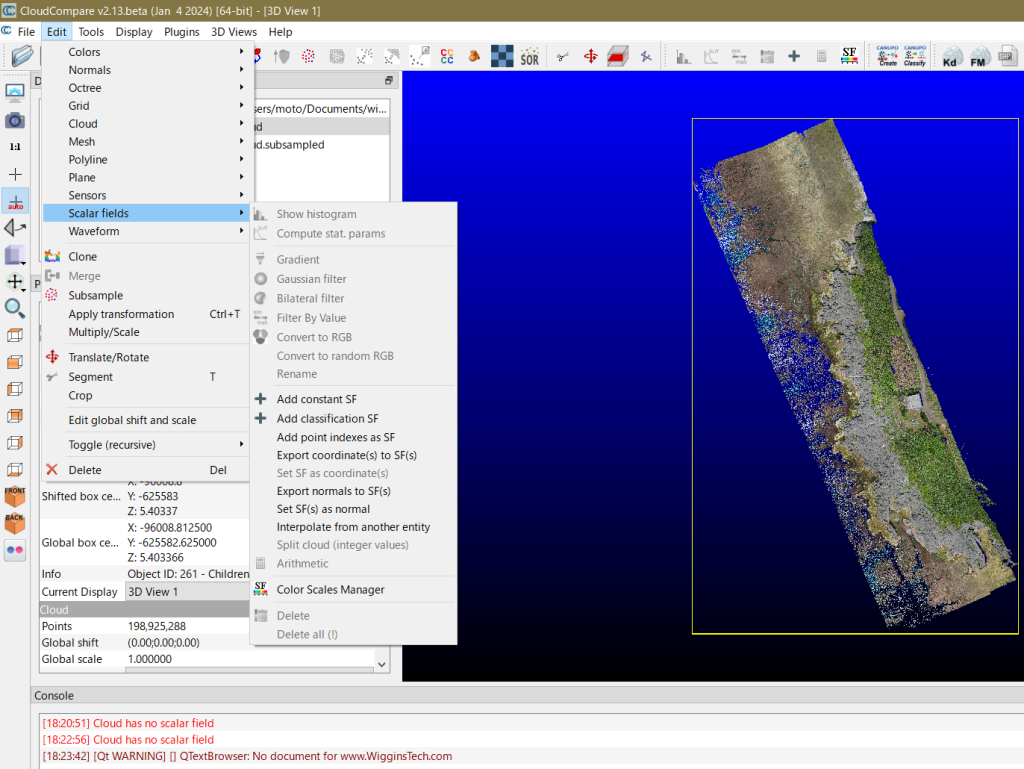
図7 Edit > Scaler fieldsのsubmenu
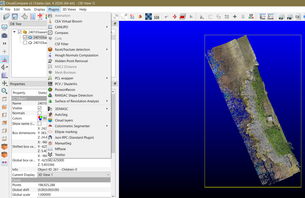
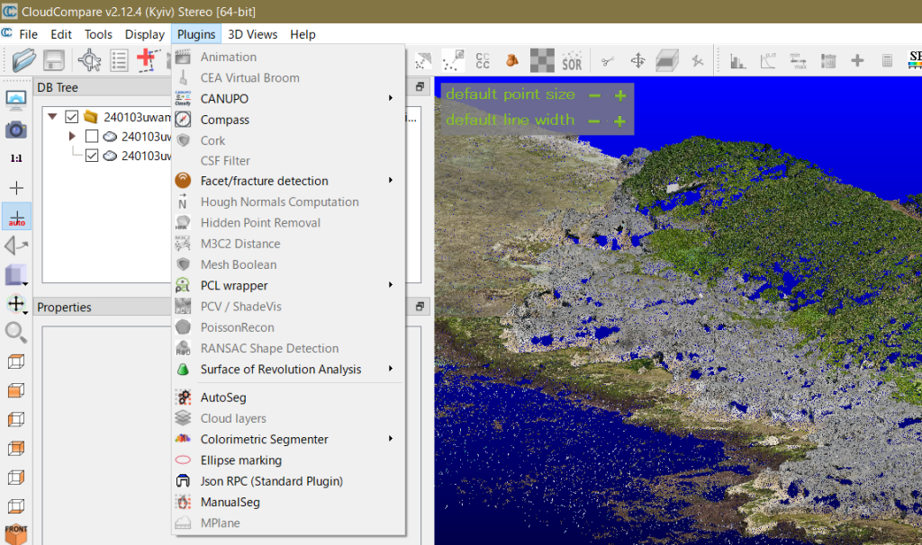
図5〜7は,新たにダウンロードしたCloudCompare v. 2.13βの表情である。CloudCompareを選択して,v. 2.12.4と比べてみた。確実に改善されている。灰色だったものがactiveになっている。図5のように,開いたPluginsの下方にCloud layersが見える。これを選択した結果が,図6で,Cloud has no scaler fieldsのエラーが現れる。図7には,Editのメニューが見えている。このScaler fieldsを選択した際のリストが見えているが,このうち,Add constant SFなどが関係しているようである。このSFは,Scaler fieldsの略号と思われ,この定義をした上で,Cloud layersを見ることができるのだろう。
次の,Edit > Cloudのうち,single point cloudしか,アクティブになっていない。もしクリップボードにデータがあれば,アクティブになる可能性がある。
‘Edit > Cloud > Create single point cloud‘
to create a cloud with a single point (set by the user)
‘Edit > Cloud > Paste from clipboard‘ (shortcut: CTRL+P)
to create a cloud from ASCII/text data stored in the clipboard
2章の末尾のDanielさんのアドバイスを次に再掲する。
Maybe you can use the new ‘qCloudLayers’ plugin? Another way, maybe more simpler, is to use the ‘Edit > Scalar fields > Split cloud (integer values)‘ method. This will create as many (sub) clouds as classes present in your cloud.
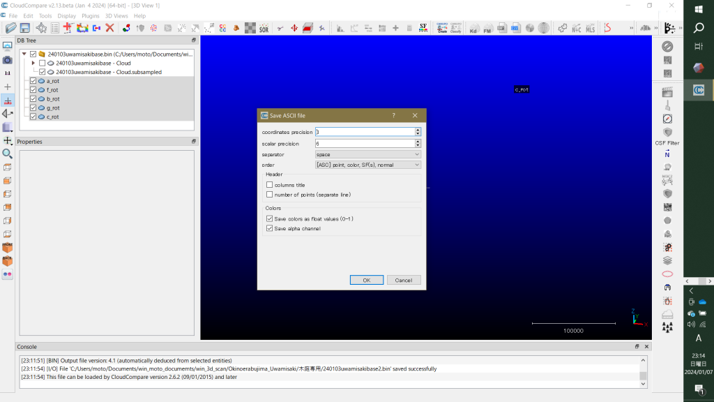
図12 Save Ascii fileパネルに適宜入力したけど。coordinate precisionを8から12に(xy座標の期待できる精度から)。Scalarは変更せず6で(a_rotなどの名称ではないかと考えては英数字6文字で十分だと)。テキストとしては扱いやすいcsvで(それでseparatorをcommaに),白いアイコンも欲しいのでColorsもそのまま。
– coordinates precision: number of digits for coordinate values (X, Y, Z) – scalar precision: number of digits for scalar field values (distance, intensity, etc.) – separator: separator character between the above values (use a comma to create a CSV file for instance) – order: order of the values (columns) – header option: to add a description header (starts with ‘//’ and then you’ll find the name of each column) – number of points: simply the total number of points on the first line (that’s expected if you want to create a valid ‘PTS’ file for some other tools) – colors: * use float values (between 0 and 1) instead of integer (between 0 and 255) for R, G and B components * save the alpha (transparency) component as well
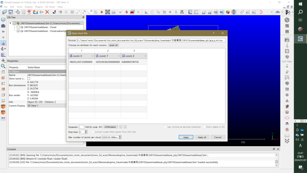
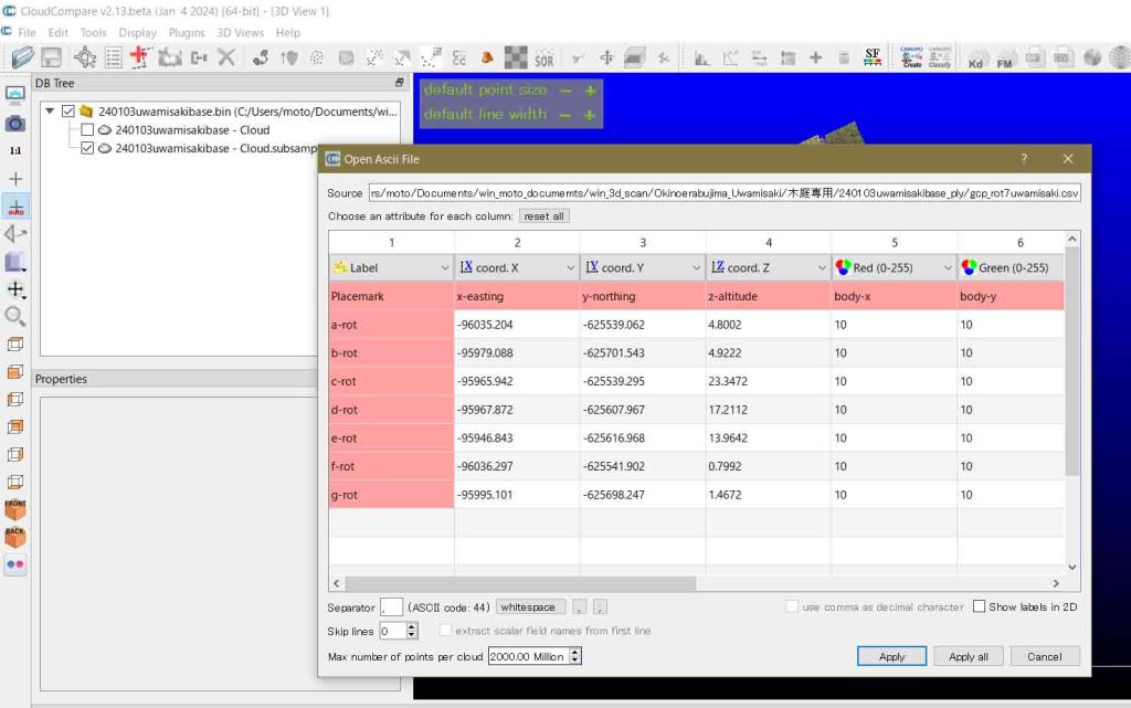
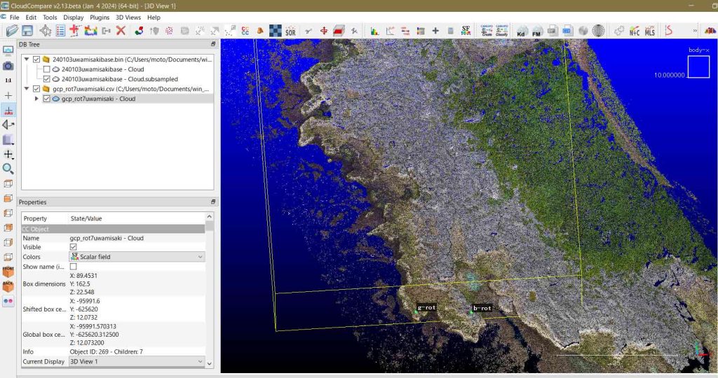
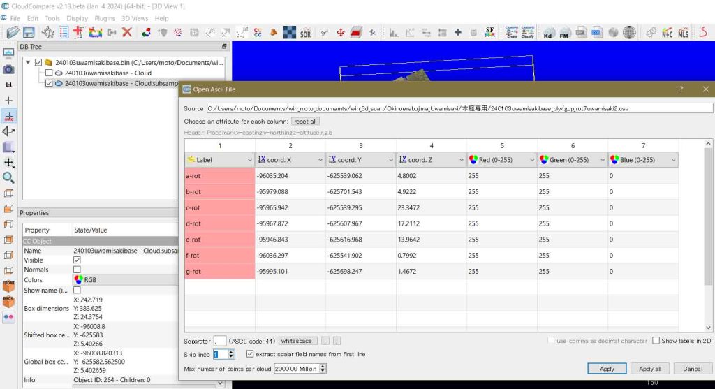
図18のように,マックのエクセルでcsvファイルを作ってウィンドウズの所定のフォルダーに入れた。それをCloudCompareで開いたら,図19のように,念願の表Open Ascii Fileが出た。これが欲しかった。やってみないとわからない。図19の葡萄茶色の行はぼくが作成した列タイトルだ。適当に,Placemark, x-easting, y-northing, z-altitude, body-x, -y, -z, R, G, Bとしたのが,このテキストから適当に解釈して,それぞれ, この葡萄茶色の行のすぐ上の灰色の行のように,Label, cood.X, Y, Z, SF Scalar 3個,Red (0-255), Green (0-255), B (0-255), と配列している。
図18 macのエクセルで作ったcsvファイルをウィンドウズに配置
図19 Open Ascii Fileが出たあ
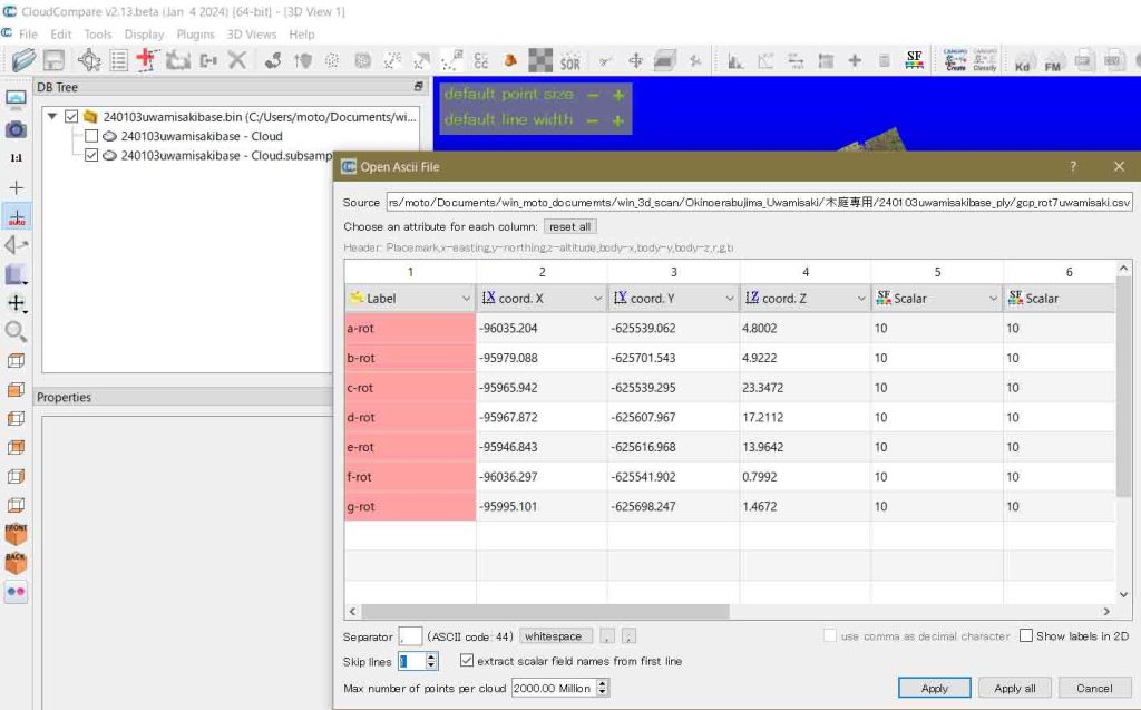
図20 タイトル行を削除
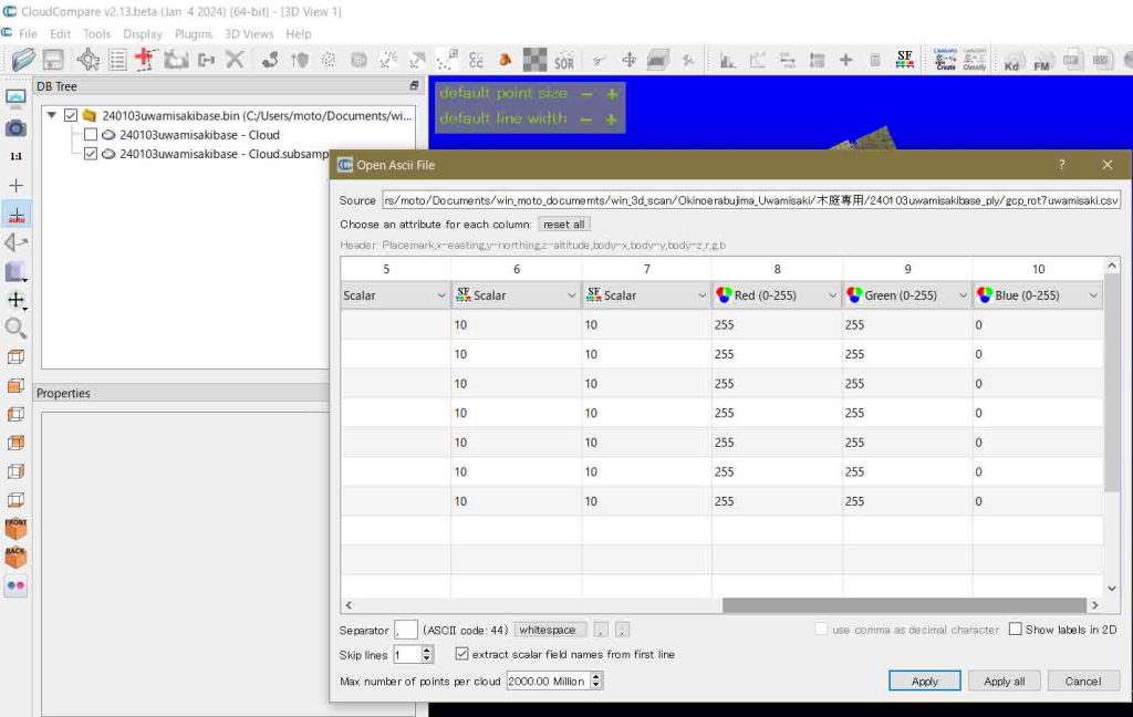
図21 図20の右方への続き
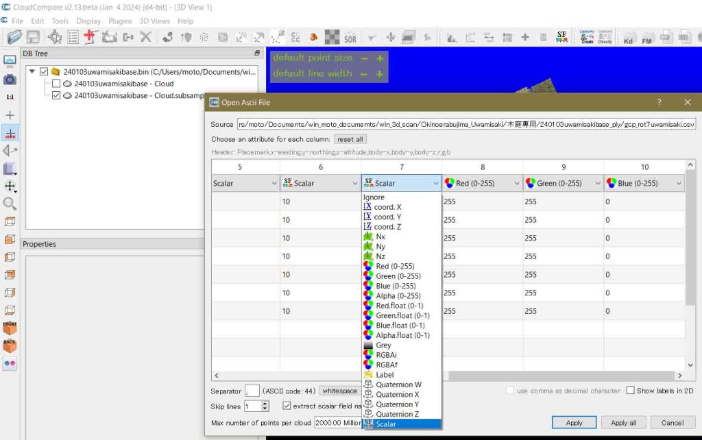
自ら設定した列タイトルに合わない場合,図22のように,変更することができる。
図22 用意された見出しを出してみた
Nx, Ny, Nzは,Per-point normal vectorsでここでは関係ない。SF-Scalarは,Per-point scalar values,であるが,ぼくはbox-xなどとしてしまったものでこれに対応している。ぼくが設定したRGBは,A unique color for the whole entityに対応しているようだ。Quaternion WXYZは複素数のようだ。とにかく,わからない。
Got it. I know Lidartools (which LAStools is dependent on) was not ported for QGIS 3 so that what I was getting at. 10M points isn’t all that big so if you have at least 16GB of RAM you shouldn’t have any problems, but considering you are having problems with a 500 point subset then we know that combined with the scaling issue that it’s probably not your plug-ins. Have you tried downloading and importing an XYZ version?
The r.in.pdal module loads PDAL library supported point clouds (with emphasis on LiDAR LAS files) into a new raster map using binning. The user may choose from a variety of statistical methods which will be used for binning when creating the new raster.
v.in.ply imports a vector map in PLY vector format. A PLY file always holds a number of vertices which are imported as points. PLY vertices can have a number of properties in addition to their coordinates. These properties are stored in an attribute table. For larger PLY files with many vertices (> 1000) it is highly recommended to not use DBF as database driver, but SQLite (default in GRASS GIS 7), PostgreSQL or MySQL, because the DBF driver is rather slow and can consume a lot of memory. The database driver can be set with db.connect.
v.in.ply is designed for large point clouds with the possibility to have only coordinates, and no attribute table (for speed reasons).
と,あって,興味深いことを次に。
GISデータの基本コンテンツと考えていたDBFが,GrassGIS7以降,デフォルトとして,使われていないことである。SQLite (default in GRASS GIS 7)。これには驚いた。ぼくは時代遅れになっていた。 上記Descriptionを見て大変期待できると思ったが,上記Notesを見ると,only coordinates, and no attribute table (for speed reasons),とあって,ショックではあった。PLYファイルからRGB情報が削除されるのである。
v.ply.rectify imports a PLY point cloud, georeferences and exports it. The first three vertex properties must be the x, y, z coordinates with property names “x”, “y”, “z”, in this order.
A text file with Ground Control Points (GCPs) must exist in the same folder where the point cloud is located, and the textfile must have the same name like the point cloud, but ending on .txt instead of .ply.
The text file with GCPs must have the following format with one GCP per line: x y z east north height status with x, y, z as source coordinates and east, north, height as target coordinates. The status indicates whether to use a GCP (status is not zero) or not (status is zero). Entries must be separated by whitespace or tabs. Decimal delimiters must be points.
The georecitifictation method used is a 3D orthogonal rectification where angles are preserved. 3D objects are shifted, scaled and rotated, but no shear is introduced. Please read the output of the module, in particular the root mean square (RMS) errors.
v.ply.rectify optionally exports the georeferenced point cloud not only with real coordinates, but also with shifted coordinates (-s flag) for display in meshlab or similar software that can not deal with real coordinates. The exported PLY point clouds will be in the same folder like the input PLY point cloud.
次の観点は重要である: x y z east north height status with x, y, z as source coordinates and east, north, height as target coordinates。通常のGISの座標系と異なり,x,y,z=easting, northing, heightになっている。別氏によればメタシェープでの処理も同様のようだ。
Create a new layer of just ground points (already classified) Joined: Tue Aug 09, 2022 10:34 am Create a new layer of just ground points (already classified) Post by okay » Tue Aug 09, 2022 10:36 am
Hi - I’m trying to make a separate layer of just the ground points in my point cloud. In other words, I want to be able to turn on and off a plot of just the ground points. I know about the CSF plug, but this isn’t necessary to use since the point cloud is classified. I can only figure out to how filter by value, but not by classification. Thanks. Location: Grenoble, France ———————————————— Contact: Contact daniel Re: Create a new layer of just ground points (already classified) Post by daniel » Wed Aug 10, 2022 5:56 pm Maybe you can use the new ‘qCloudLayers’ plugin? Another way, maybe more simpler, is to use the ‘Edit > Scalar fields > Split cloud (integer values)’ method. This will create as many (sub) clouds as classes present in your cloud. Daniel, CloudCompare admin ————————————————